31

I am trying to get a better understanding of kernel density estimation.

Using the definition from Wikipedia: https://en.wikipedia.org/wiki/Kernel_density_estimation#Definition

$ \hat{f_h}(x) = \frac{1}{n}\sum_{i=1}^n K_h (x - x_i) \quad = \frac{1}{nh} \sum_{i=1}^n K\Big(\frac{x-x_i}{h}\Big) $

Let's take $K()$ to be a rectangular function which gives $1$ if $x$ is between $-0.5$ and $0.5$ and $0$ otherwise, and $h$ (window size) to be 1.

I understand that the density is a convolution of two functions, but I am not sure I know how to define these two functions. One of them should (probably) be a function of the data which, for every point in R, tells us how many data points we have in that location (mostly $0$). And the other function should probably be some modification of the kernel function, combined with the window size. But I am not sure how to define it.

Any suggestions?

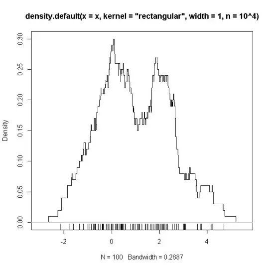
Bellow is an example R code which (I suspect) replicates the settings I defined above (with a mixture of two Gaussians and $n=100$), on which I hope to see a "proof" that the functions to be convoluted are as we suspect.

# example code:
set.seed(2346639)
x <- c(rnorm(50), rnorm(50,2))
plot(density(x, kernel='rectangular', width=1, n = 10**4))
rug(x)

enter image description here

Danica
  • 21,852
  • 1
  • 59
  • 115
Tal Galili
  • 19,935
  • 32
  • 133
  • 195
  • 3
    Your rug at the bottom gives some rough intuition. Imagine each value $x_i$ from $i = 1$ to $n$ is a spike with an associated weight $1/n$. Now smear each spike using the shape and width of your kernel, so that the spike is transformed to take on the same shape and width, with a height such that the area below is $1/n$. Add the results and you have a kernel density estimate. – Nick Cox Oct 23 '13 at 19:57
  • Hi Nick, thank you for the comment. This far in the intuition I already got, it is the turning it formally into the form of the convolution which I was curious to see :) (I'm eager to now go through Whuber's answer!) – Tal Galili Oct 23 '13 at 20:07

1 Answers1

32

Corresponding to any batch of data $X = (x_1, x_2, \ldots, x_n)$ is its "empirical density function"

$$f_X(x) = \frac{1}{n}\sum_{i=1}^{n} \delta(x-x_i).$$

Here, $\delta$ is a "generalized function." Despite that name, it isn't a function at all: it's a new mathematical object that can be used only within integrals. Its defining property is that for any function $g$ of compact support that is continuous in a neighborhood of $0$,

$$\int_{\mathbb{R}}\delta(x) g(x) dx = g(0).$$

(Names for $\delta$ include "atomic" or "point" measure and "Dirac delta function." In the following calculation this concept is extended to include functions $g$ which are continuous from one side only.)

Justifying this characterization of $f_X$ is the observation that

$$\eqalign{ \int_{-\infty}^{x} f_X(y) dy &= \int_{-\infty}^{x} \frac{1}{n}\sum_{i=1}^{n} \delta(y-x_i)dy \\ &= \frac{1}{n}\sum_{i=1}^{n} \int_{-\infty}^{x} \delta(y-x_i)dy \\ &= \frac{1}{n}\sum_{i=1}^{n} \int_{\mathbb{R}} I(y\le x) \delta(y-x_i)dy \\ &= \frac{1}{n}\sum_{i=1}^{n} I(x_i \le x) \\ &= F_X(x) }$$

where $F_X$ is the usual empirical CDF and $I$ is the usual characteristic function (equal to $1$ where its argument is true and $0$ otherwise). (I skip an elementary limiting argument needed to move from functions of compact support to functions defined over $\mathbb{R}$; because $I$ only needs to be defined for values within the range of $X$, which is compact, this is no problem.)

The convolution of $f_X(x)$ with any other function $k$ is given, by definition, as

$$\eqalign{ (f_X * k)(x) &= \int_{\mathbb{R}} f_X(x - y) k(y) dy \\ &=\int_{\mathbb{R}} \frac{1}{n}\sum_{i=1}^{n} \delta(x-y-x_i) k(y) dy \\ &= \frac{1}{n}\sum_{i=1}^{n}\int_{\mathbb{R}} \delta(x-y-x_i) k(y) dy \\ &=\frac{1}{n}\sum_{i=1}^{n} k(x_i-x). }$$

Letting $k(x) = K_h(-x)$ (which is the same as $K_h(x)$ for symmetric kernels--and most kernels are symmetric) we obtain the claimed result: the Wikipedia formula is a convolution.

whuber
  • 281,159
  • 54
  • 637
  • 1,101
  • 1
    The situation in two dimensions is explained (in more colloquial terms) and illustrated on the GIS site at http://gis.stackexchange.com/questions/14374/interpretation-of-arcgis-kernel-density-legend-parameters/14376#14376. – whuber Oct 23 '13 at 20:04
  • 2
    Dear Whuber, I just went through and read your answer with delight! Thank you very much for the explanation and details, your answers (this one, and your others in general) are truly inspiring. Yours, Tal – Tal Galili Oct 23 '13 at 20:28
  • 1
    I think this is called a Dirac comb. – Elvis Oct 24 '13 at 05:25
  • 1
    @Elvis According to [Wikipedia](http://en.wikipedia.org/wiki/Dirac_comb), a Dirac comb corresponds to a *periodic* (and therefore infinite) set of data. Although the machinery is similar, the concept does not appear to apply to this question. – whuber Oct 24 '13 at 05:31
  • Hi, nice answer. I do not understand one thing though. Do we treat the input of the dirac measure as a one-point set? How would we write the above computations if we did not abuse the notation? – Jan Vainer May 19 '19 at 08:16
  • @Jan AFAIK, there is no abuse of notation: $\delta$ is a generalized function in the sense I gave at the outset. See https://en.wikipedia.org/wiki/Generalized_function#Schwartz_distributions for a brief account. – whuber May 19 '19 at 13:06
  • @whuber Thank you for swift response. Do I understand it correctly, that the empirical density's value $f(x)$ is simply the fraction of points from the sample that attain value $x$? Could you please briefly elaborate on the difference between the dirac function and an indicator function in this context? (I understand that the integral of indicator function would be zero, but in the first sum of your answer they seem the same to me). I can open a new qustion for it if you wish. – Jan Vainer May 19 '19 at 13:32
  • 1
    @Jan Your understanding is not quite correct. There is no empirical "density" in the sense of a finite continuous measure. The indicator function of the data integrates to zero (whether you use Lebesgue integration or Riemann integration makes no difference). The generalized function $\delta$ is not a function at all: it's a new mathematical object that can be used only within integrals. The empirical *distribution* is a mathematical object that, when integrated against any integrable function $g,$ returns the sum (over all data $x_i$) of the values $g(x_i).$ – whuber May 19 '19 at 13:41
  • 1
    @whuber Thank you. The sentence *The generalized function δ is not a function at all: it's a new mathematical object that can be used only within integrals.* made it clearer. on point as always. ;) – Jan Vainer May 19 '19 at 14:05
  • 1
    @Jan Thank you for your help: I have incorporated that idea within this answer. – whuber May 19 '19 at 14:28
  • For those struggling with the Dirac-delta function, I wrote a blog post about it. I explain what the Dirac-delta function is and how it can be used for sampling, [here](https://maurocamaraescudero.netlify.app/post/towards-smc-using-the-dirac-delta-function-in-sampling-and-sequential-monte-carlo/) – Euler_Salter May 19 '20 at 15:38
  • 1
    @Euler Please note that $\delta$ is not a function and it is not differentiable at $0.$ It can be conceived of either as a *generalized function* or a *measure.* In the former sense it does have a derivative--but that derivative is not infinite at zero; it is another generalized function (one that returns the negative derivative of any differentiable function against which it is integrated). – whuber May 19 '20 at 15:45