Understanding an empirical distribution defined by a Dirac measure

Question

There is a definition in this paper (equation 2.3) which I cannot seem to grasp. I'm writing it here in a simpler form:

Let $\delta_a$ be the Dirac measure which assigns probability 1 to the point $a$. Denote measure $\mu \in \mathcal{P}_{ac}(R^d)$ where $\mathcal{P}_{ac}(R^d)$ is the family of all Lebesgue absolutely continuous probability measures on $R^d$. Let $\boldsymbol{X}$ be a random vector, and its empirical observations are $\boldsymbol{X}_1, \boldsymbol{X}_2, ..., \boldsymbol{X}_n\ \stackrel{i.i.d.}{\sim}\ \mu \in \mathcal{P}_{ac}(R^d)$.

Now, in the paper they define the empirical distribution of $\boldsymbol{X}$ as: $$\mu_n^{\boldsymbol{X}} := \frac{1}{n} \sum_{i=1}^n \delta_{\boldsymbol{X}_i},$$

and this is the part I don't get. How does the above sum represent an empirical distribution? is it actually like saying the observations are uniformly distributed because for each observation the value of the above sum will be $1/n$?

Answer 1

is it actually like saying the observations are uniformly distributed because for each observation the value of the above sum will be $1/$?

Not really. The distribution would be uniform if the observed values would be uniformly distributed. The empirical distribution would depend on observed data, so if you observed the values $(1, 1, 3)$, the probability for $1$ would be $2/3$ rather than $1/3$ since there’s sum involved.

Answer 2

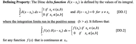
In the paper, it states that $\delta_a$ refers to a Dirac delta at the "point" $a$. In other words: which means that the value of 1 (i.e., one event) occurs is some space (e.g., 1D, 2D, 3D...), and is at a point coordinate "$a$" in that whatever it is space. Now as "events" or more generally "data" accumulates accumulates in that space, each event contributes $\frac{1}{n}$, to the ensemble, or total number of points such that each event, even though 100% probably at that point, is only one of $n$ others, such that post hoc each event was only $p=\frac{1}{n}$ of all observations.

Example: We take a drop of concentrated NaF-18 (positron emitting F-18 as sodium fluoride in aqueous solution) and drop in into a cubic water bath that is located within a PET (positron emission tomography) 3D scanner. We collect events [positron-electron (matter antimatter) annihilation events detected as dual 511 keV coincidence photons] each of which is 100% probable when it occurs. We reconstruct a list of events in time and their positions in 3-space, and do so for an extended time. This forms a 4D image sequence which if we watch it as a movie shows a small object eventually circulating with a tenancy of becoming uniformly distributed due to fluid mixing from any convection currents within the water bath and diffusion within that fluid.

Now instead of a discrete distribution let's make a pseudo-continuous model. We do the same thing again only this time with a drop of India ink. The ink will eventually mix within the water bath, and we just use our eyes to look at it. The image we see looks continuous, but actually, in a very dark room, if you look carefully, you can see individual spots of light that are single photons, i.e., we think that our 4D mixing of ink is continuous, but actually it is only approximately continuous as the number of events is so large that we see a spaciotemporally smoothed image.

Now, let's make a 5D object. We take blue ink and yellow ink and put a drop of each a few cm apart in a clear water bath. Eventually these mix and the bath, assuming we are not Daltonists (i.e., those with red-green color blindness), will turn green. Now we have two independent types of Dirac delta's; from blue and yellow photons. So, in review, our 5 dimensions were color, time, and three space, and each "point" had 5 coordinates in color-space-time.

Answer 3

It's easiest to think backwards: integrate this PDF (measure) to get to CDF.

For instance, consider PDF $f(X)=(\delta(x)+\delta(x-1))/2$, then integrate to get CDF $$F(x)=\int_{-\infty}^x f(s)ds$$ This CDF is step function with $F(X<0)=0$, $F(0\le x<1)=1/2$ and $F(1\le X)=1$. This is your empirical CDF.

Once you get this one dimensional case then it's easy to extend the intuition to multi-dimensional case that you have. It's a mechanical application of integration, even if it's Lebesgue, the idea's the same.

If you were a physicist then you'd know how Dirac came up with his function: a continuous analogue of the Kroneker delta function, i.e. spiritually the same idea of representing discrete points in continuous function analysis.