Relationship between SVD and PCA. How to use SVD to perform PCA?

Question

Principal component analysis (PCA) is usually explained via an eigen-decomposition of the covariance matrix. However, it can also be performed via singular value decomposition (SVD) of the data matrix $\mathbf X$. How does it work? What is the connection between these two approaches? What is the relationship between SVD and PCA?

Or in other words, how to use SVD of the data matrix to perform dimensionality reduction?

Answer 1

Let the data matrix $\mathbf X$ be of $n \times p$ size, where $n$ is the number of samples and $p$ is the number of variables. Let us assume that it is centered, i.e. column means have been subtracted and are now equal to zero.

Then the $p \times p$ covariance matrix $\mathbf C$ is given by $\mathbf C = \mathbf X^\top \mathbf X/(n-1)$. It is a symmetric matrix and so it can be diagonalized: $$\mathbf C = \mathbf V \mathbf L \mathbf V^\top,$$ where $\mathbf V$ is a matrix of eigenvectors (each column is an eigenvector) and $\mathbf L$ is a diagonal matrix with eigenvalues $\lambda_i$ in the decreasing order on the diagonal. The eigenvectors are called principal axes or principal directions of the data. Projections of the data on the principal axes are called principal components, also known as PC scores; these can be seen as new, transformed, variables. The $j$-th principal component is given by $j$-th column of $\mathbf {XV}$. The coordinates of the $i$-th data point in the new PC space are given by the $i$-th row of $\mathbf{XV}$.

If we now perform singular value decomposition of $\mathbf X$, we obtain a decomposition $$\mathbf X = \mathbf U \mathbf S \mathbf V^\top,$$ where $\mathbf U$ is a unitary matrix and $\mathbf S$ is the diagonal matrix of singular values $s_i$. From here one can easily see that $$\mathbf C = \mathbf V \mathbf S \mathbf U^\top \mathbf U \mathbf S \mathbf V^\top /(n-1) = \mathbf V \frac{\mathbf S^2}{n-1}\mathbf V^\top,$$ meaning that right singular vectors $\mathbf V$ are principal directions and that singular values are related to the eigenvalues of covariance matrix via $\lambda_i = s_i^2/(n-1)$. Principal components are given by $\mathbf X \mathbf V = \mathbf U \mathbf S \mathbf V^\top \mathbf V = \mathbf U \mathbf S$.

To summarize:

1. If $\mathbf X = \mathbf U \mathbf S \mathbf V^\top$, then columns of $\mathbf V$ are principal directions/axes.
2. Columns of $\mathbf {US}$ are principal components ("scores").
3. Singular values are related to the eigenvalues of covariance matrix via $\lambda_i = s_i^2/(n-1)$. Eigenvalues $\lambda_i$ show variances of the respective PCs.
4. Standardized scores are given by columns of $\sqrt{n-1}\mathbf U$ and loadings are given by columns of $\mathbf V \mathbf S/\sqrt{n-1}$. See e.g. here and here for why "loadings" should not be confused with principal directions.
5. The above is correct only if $\mathbf X$ is centered. Only then is covariance matrix equal to $\mathbf X^\top \mathbf X/(n-1)$.
6. The above is correct only for $\mathbf X$ having samples in rows and variables in columns. If variables are in rows and samples in columns, then $\mathbf U$ and $\mathbf V$ exchange interpretations.
7. If one wants to perform PCA on a correlation matrix (instead of a covariance matrix), then columns of $\mathbf X$ should not only be centered, but standardized as well, i.e. divided by their standard deviations.
8. To reduce the dimensionality of the data from $p$ to $k<p$, select $k$ first columns of $\mathbf U$, and $k\times k$ upper-left part of $\mathbf S$. Their product $\mathbf U_k \mathbf S_k$ is the required $n \times k$ matrix containing first $k$ PCs.
9. Further multiplying the first $k$ PCs by the corresponding principal axes $\mathbf V_k^\top$ yields $\mathbf X_k = \mathbf U_k^\vphantom \top \mathbf S_k^\vphantom \top \mathbf V_k^\top$ matrix that has the original $n \times p$ size but is of lower rank (of rank $k$). This matrix $\mathbf X_k$ provides a reconstruction of the original data from the first $k$ PCs. It has the lowest possible reconstruction error, see my answer here.
10. Strictly speaking, $\mathbf U$ is of $n\times n$ size and $\mathbf V$ is of $p \times p$ size. However, if $n>p$ then the last $n-p$ columns of $\mathbf U$ are arbitrary (and corresponding rows of $\mathbf S$ are constant zero); one should therefore use an economy size (or thin) SVD that returns $\mathbf U$ of $n\times p$ size, dropping the useless columns. For large $n\gg p$ the matrix $\mathbf U$ would otherwise be unnecessarily huge. The same applies for an opposite situation of $n\ll p$.

---

Further links

• What is the intuitive relationship between SVD and PCA -- a very popular and very similar thread on math.SE.

• Why PCA of data by means of SVD of the data? -- a discussion of what are the benefits of performing PCA via SVD [short answer: numerical stability].

• PCA and Correspondence analysis in their relation to Biplot -- PCA in the context of some congeneric techniques, all based on SVD.

• Is there any advantage of SVD over PCA? -- a question asking if there any benefits in using SVD instead of PCA [short answer: ill-posed question].

• Making sense of principal component analysis, eigenvectors & eigenvalues -- my answer giving a non-technical explanation of PCA. To draw attention, I reproduce one figure here:

Answer 2

I wrote a Python & Numpy snippet that accompanies @amoeba's answer and I leave it here in case it is useful for someone. The comments are mostly taken from @amoeba's answer.

import numpy as np
from numpy import linalg as la
np.random.seed(42)


def flip_signs(A, B):
    """
    utility function for resolving the sign ambiguity in SVD
    http://stats.stackexchange.com/q/34396/115202
    """
    signs = np.sign(A) * np.sign(B)
    return A, B * signs


# Let the data matrix X be of n x p size,
# where n is the number of samples and p is the number of variables
n, p = 5, 3
X = np.random.rand(n, p)
# Let us assume that it is centered
X -= np.mean(X, axis=0)

# the p x p covariance matrix
C = np.cov(X, rowvar=False)
print "C = \n", C
# C is a symmetric matrix and so it can be diagonalized:
l, principal_axes = la.eig(C)
# sort results wrt. eigenvalues
idx = l.argsort()[::-1]
l, principal_axes = l[idx], principal_axes[:, idx]
# the eigenvalues in decreasing order
print "l = \n", l
# a matrix of eigenvectors (each column is an eigenvector)
print "V = \n", principal_axes
# projections of X on the principal axes are called principal components
principal_components = X.dot(principal_axes)
print "Y = \n", principal_components

# we now perform singular value decomposition of X
# "economy size" (or "thin") SVD
U, s, Vt = la.svd(X, full_matrices=False)
V = Vt.T
S = np.diag(s)

# 1) then columns of V are principal directions/axes.
assert np.allclose(*flip_signs(V, principal_axes))

# 2) columns of US are principal components
assert np.allclose(*flip_signs(U.dot(S), principal_components))

# 3) singular values are related to the eigenvalues of covariance matrix
assert np.allclose((s ** 2) / (n - 1), l)

# 8) dimensionality reduction
k = 2
PC_k = principal_components[:, 0:k]
US_k = U[:, 0:k].dot(S[0:k, 0:k])
assert np.allclose(*flip_signs(PC_k, US_k))

# 10) we used "economy size" (or "thin") SVD
assert U.shape == (n, p)
assert S.shape == (p, p)
assert V.shape == (p, p)

Answer 3

Let me start with PCA. Suppose that you have n data points comprised of d numbers (or dimensions) each. If you center this data (subtract the mean data point $\mu$ from each data vector $x_i$) you can stack the data to make a matrix

$$ X = \left( \begin{array}{ccccc} && x_1^T - \mu^T && \\ \hline && x_2^T - \mu^T && \\ \hline && \vdots && \\ \hline && x_n^T - \mu^T && \end{array} \right)\,. $$

The covariance matrix

$$ S = \frac{1}{n-1} \sum_{i=1}^n (x_i-\mu)(x_i-\mu)^T = \frac{1}{n-1} X^T X $$

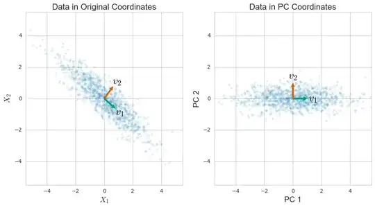
measures to which degree the different coordinates in which your data is given vary together. So, it's maybe not surprising that PCA -- which is designed to capture the variation of your data -- can be given in terms of the covariance matrix. In particular, the eigenvalue decomposition of $S$ turns out to be

$$ S = V \Lambda V^T = \sum_{i = 1}^r \lambda_i v_i v_i^T \,, $$

where $v_i$ is the $i$-th Principal Component, or PC, and $\lambda_i$ is the $i$-th eigenvalue of $S$ and is also equal to the variance of the data along the $i$-th PC. This decomposition comes from a general theorem in linear algebra, and some work does have to be done to motivate the relatino to PCA.

SVD is a general way to understand a matrix in terms of its column-space and row-space. (It's a way to rewrite any matrix in terms of other matrices with an intuitive relation to the row and column space.) For example, for the matrix $A = \left( \begin{array}{cc}1&2\\0&1\end{array} \right)$ we can find directions $u_i$ and $v_i$ in the domain and range so that

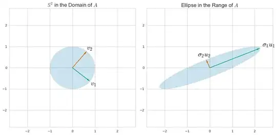
You can find these by considering how $A$ as a linear transformation morphs a unit sphere $\mathbb S$ in its domain to an ellipse: the principal semi-axes of the ellipse align with the $u_i$ and the $v_i$ are their preimages.

In any case, for the data matrix $X$ above (really, just set $A = X$), SVD lets us write

$$ X = \sum_{i=1}^r \sigma_i u_i v_j^T\,, $$

where $\{ u_i \}$ and $\{ v_i \}$ are orthonormal sets of vectors.A comparison with the eigenvalue decomposition of $S$ reveals that the "right singular vectors" $v_i$ are equal to the PCs, the "right singular vectors" are

$$ u_i = \frac{1}{\sqrt{(n-1)\lambda_i}} Xv_i\,, $$

and the "singular values" $\sigma_i$ are related to the data matrix via

$$ \sigma_i^2 = (n-1) \lambda_i\,. $$

It's a general fact that the right singular vectors $u_i$ span the column space of $X$. In this specific case, $u_i$ give us a scaled projection of the data $X$ onto the direction of the $i$-th principal component. The left singular vectors $v_i$ in general span the row space of $X$, which gives us a set of orthonormal vectors that spans the data much like PCs.

I go into some more details and benefits of the relationship between PCA and SVD in this longer article.