29

I am trying to perform a multiple regression in R. However, my dependent variable has the following plot:

DV

Here is a scatterplot matrix with all my variables (WAR is the dependent variable):

SPLOM

I know that I need to perform a transformation on this variable (and possibly the independent variables?) but I am not sure of the exact transformation required. Can someone point me in the right direction? I am happy to provide any additional information about the relationship between the independent and dependent variables.

The diagnostic graphics from my regression look as follows:

Diagnostic plots

EDIT

After transforming the dependent and independent variables using Yeo-Johnson transformations, the diagnostic plots look like this:

After transforming

If I use a GLM with a log-link, the diagnostic graphics are:

GLM with log-link

COOLSerdash
  • 25,317
  • 8
  • 73
  • 123
zgall1
  • 809
  • 2
  • 13
  • 17
  • 4
    Hi @zglaa1 and welcome. Why do you think that you have to transform the variables? The first step would be to fit the regression with the original varibales and then look at the fit (residuals etc.). The residuals should approximately normally distributed, not the variables. Maybe you'll find [this post](http://stats.stackexchange.com/questions/33392/improving-transformation-of-dependent-variable-and-robust-regression?rq=1) interesting. – COOLSerdash Jun 08 '13 at 13:26
  • Thank for you for both the link and the suggestion. I have run my regression and I know the variables need to be transformed based on the following plot: http://i.imgur.com/rbmu14M.jpg I can see unbiasedness and lack of constant variability in the residuals. Also, they are not normal. – zgall1 Jun 08 '13 at 13:40
  • @COOLSerdash I took a look at the link. I have a basic background in statistics so I understand the discussion. However, my problem is that I have limited experience with actually applying the techniques I have learned so I struggle to figure out what exactly I need to do with my data (either in Excel or R) to actually perform the necessary transformations. – zgall1 Jun 08 '13 at 13:45
  • Thanks for the graphic. You are absolutely right by saying that this fit is suboptimal. Could you please produce a scatterplot matrix with the DV and IVs in the regression? This can be done in `R` with the command `pairs(my.data, lower.panel = panel.smooth)` where `my.data` would be your dataset. – COOLSerdash Jun 08 '13 at 13:49
  • @COOLSerdash Here you go - http://i.imgur.com/k9LFsP4.jpg You'll notice there are 5 dummy variables. I can remove them if they make reading the scatterplot easier. – zgall1 Jun 08 '13 at 13:59
  • As @Nick recommended in his answer, you might try a GLM with a log-link. In `R`, this can be achieved by typing: `my.mod – COOLSerdash Jun 08 '13 at 14:14
  • 2
    A general approach to transformation are [Box-Cox transformations](http://en.wikipedia.org/wiki/Power_transform#Box.E2.80.93Cox_transformation). What you could do is the following: 1. Fit your regression model with `lm` using the untransformed variables. 2. Use the function `boxcox(my.lm.model)` from the `MASS` package to estimate $\lambda$. The command also produces a graphic that you could upload for our convenience. – COOLSerdash Jun 08 '13 at 14:26
  • @COOLSerdash Here is the boxcox graphic. Would you be able to explain how exactly take the boxcox transformation data, specifically the λ value, and use it to transform my data? – zgall1 Jun 08 '13 at 14:56
  • What does the Box-Cox function in MASS do with zero and negative values? Note that the Wikipedia link does explain what $\lambda$ is. – Nick Cox Jun 08 '13 at 15:06
  • I wish I could understand that Wikipedia link. With regards to the zero and negative values, I simply re-coded them as 0.000001. While I'm sure you will hate that, I have strong reasons to believe that this will have absolutely no impact on the model. As you said you had no interest in baseball minutiae, I will refrain from explaining my rationale. – zgall1 Jun 08 '13 at 15:14
  • @COOLSerdash These are the diagnostic graphs after running the GLM with log-link. It looks better but there are still clearly some issues. http://i.imgur.com/FjjAdoW.jpg – zgall1 Jun 08 '13 at 15:15
  • You are correct; I recommend against that. Quite apart from not respecting the data, you just created lots of massive outliers on the logarithmic scale. A very, very small value instead of zero is _not_ a conservative change; it's a drastic one! I don't mean to be offensive about baseball; I just won't understand your rationale. But what you just did is statistically inadvisable, regardless of the nature of the data. – Nick Cox Jun 08 '13 at 15:19
  • I will edit my answer to expand on the previous comment. – Nick Cox Jun 08 '13 at 15:21
  • Nick - I appreciate your fuller explanation. I will try the GLM with log-link using the original data set. The Box-Cox function doesn't appear to work with negative values or zeros (as you hinted at) and I'm not aware of an alternative function. – zgall1 Jun 08 '13 at 15:25
  • I tried the GLM with log-link using the original data set and received the following error: Error in eval(expr, envir, enclos) : cannot find valid starting values: please specify some I did some searching and found the following link that mentions this problem - http://stackoverflow.com/questions/8212063/r-glm-starting-values-not-accepted-log-link - but was not able to figure out how to apply the suggestions to my particular problem. Any help would be appreciated. – zgall1 Jun 08 '13 at 15:27
  • I don't use R routinely, so you need help from someone accustomed to GLM in R. – Nick Cox Jun 08 '13 at 15:33
  • Because your first diagnostic plot shows distinct lack of fit in the mean, the other plots aren't particularly informative; it's hard to disentangle a problem in those plots from the already identified model failure. Your GLM results suggest using a model with a different variance-function – Glen_b Jun 09 '13 at 06:17
  • Could you elaborate on what you mean by a different variance function? – zgall1 Jun 09 '13 at 21:53

2 Answers2

34

John Fox's book An R companion to applied regression is an excellent ressource on applied regression modelling with R. The package car which I use throughout in this answer is the accompanying package. The book also has as website with additional chapters.


Transforming the response (aka dependent variable, outcome)

Box-Cox transformations offer a possible way for choosing a transformation of the response. After fitting your regression model containing untransformed variables with the R function lm, you can use the function boxCox from the car package to estimate $\lambda$ (i.e. the power parameter) by maximum likelihood. Because your dependent variable isn't strictly positive, Box-Cox transformations will not work and you have to specify the option family="yjPower" to use the Yeo-Johnson transformations (see the original paper here and this related post):

boxCox(my.regression.model, family="yjPower", plotit = TRUE)

This produces a plot like the following one:

Box-Cox lambdaplot

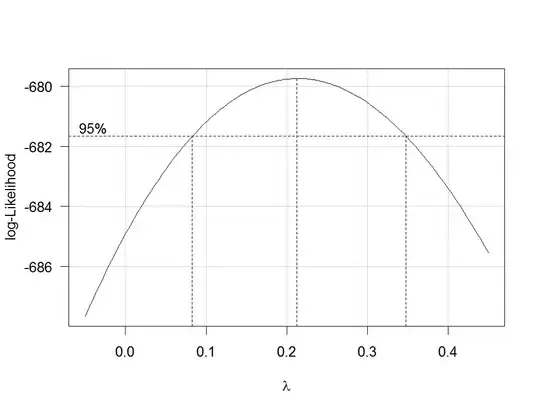
The best estimate of $\lambda$ is the value that maximizes the profile likelhod which in this example is about 0.2. Usually, the estimate of $\lambda$ is rounded to a familiar value that is still within the 95%-confidence interval, such as -1, -1/2, 0, 1/3, 1/2, 1 or 2.

To transform your dependent variable now, use the function yjPower from the car package:

depvar.transformed <- yjPower(my.dependent.variable, lambda)

In the function, the lambda should be the rounded $\lambda$ you have found before using boxCox. Then fit the regression again with the transformed dependent variable.

Important: Rather than just log-transform the dependent variable, you should consider to fit a GLM with a log-link. Here are some references that provide further information: first, second, third. To do this in R, use glm:

glm.mod <- glm(y~x1+x2, family=gaussian(link="log"))

where y is your dependent variable and x1, x2 etc. are your independent variables.


Transformations of predictors

Transformations of strictly positive predictors can be estimated by maximum likelihood after the transformation of the dependent variable. To do so, use the function boxTidwell from the car package (for the original paper see here). Use it like that: boxTidwell(y~x1+x2, other.x=~x3+x4). The important thing here is that option other.x indicates the terms of the regression that are not to be transformed. This would be all your categorical variables. The function produces an output of the following form:

boxTidwell(prestige ~ income + education, other.x=~ type + poly(women, 2), data=Prestige)

          Score Statistic   p-value MLE of lambda
income          -4.482406 0.0000074    -0.3476283
education        0.216991 0.8282154     1.2538274

In that case, the score test suggests that the variable income should be transformed. The maximum likelihood estimates of $\lambda$ for income is -0.348. This could be rounded to -0.5 which is analogous to the transformation $\text{income}_{new}=1/\sqrt{\text{income}_{old}}$.

Another very interesting post on the site about the transformation of the independent variables is this one.


Disadvantages of transformations

While log-transformed dependent and/or independent variables can be interpreted relatively easy, the interpretation of other, more complicated transformations is less intuitive (for me at least). How would you, for example, interpret the regression coefficients after the dependent variables has been transformed by $1/\sqrt{y}$? There are quite a few posts on this site that deal exactly with that question: first, second, third, fourth. If you use the $\lambda$ from Box-Cox directly, without rounding (e.g. $\lambda$=-0.382), it is even more difficult to interpret the regression coefficients.


Modelling nonlinear relationships

Two quite flexible methods to fit nonlinear relationships are fractional polynomials and splines. These three papers offer a very good introduction to both methods: First, second and third. There is also a whole book about fractional polynomials and R. The R package mfp implements multivariable fractional polynomials. This presentation might be informative regarding fractional polynomials. To fit splines, you can use the function gam (generalized additive models, see here for an excellent introduction with R) from the package mgcv or the functions ns (natural cubic splines) and bs (cubic B-splines) from the package splines (see here for an example of the usage of these functions). Using gam you can specify which predictors you want to fit using splines using the s() function:

my.gam <- gam(y~s(x1) + x2, family=gaussian())

here, x1 would be fitted using a spline and x2 linearly as in a normal linear regression. Inside gam you can specify the distribution family and the link function as in glm. So to fit a model with a log-link function, you can specify the option family=gaussian(link="log") in gam as in glm.

Have a look at this post from the site.

COOLSerdash
  • 25,317
  • 8
  • 73
  • 123
  • 1
    Good explanation. I don't know that explicit Box-Cox is really the most common method of choosing a transformation. If you count people who just choose logs any way, my own wild guess is that it's a minority method. That picky point doesn't affect anything else, naturally. – Nick Cox Jun 08 '13 at 15:39
  • @NickCox Thanks (+1 for your answer, btw). The statement that Box-Cox is the most common method comes from John Fox's book. I took it at face value as I don't have enough experience to judge the statement. I'll remove the statement. – COOLSerdash Jun 08 '13 at 15:44
  • Thank you so much for the detailed explanation. I will try and apply it to my data now. – zgall1 Jun 08 '13 at 15:46
  • @COOLSerdash Using your detailed walkthrough, I applied the Box Cox transformation to my dependent and then independent variables and have the following plot of my diagnostic variables - http://i.imgur.com/eO01djl.jpg Clearly, there is an improvement but there still seems to be issues with constant variability and unbiasedness and there is definitely an issue with normality. Where can I go from here? – zgall1 Jun 08 '13 at 16:52
  • @COOLSerdash I also tried the GLM method and got the following - http://i.imgur.com/FjjAdoW.jpg The same comment as the one above applies. There is a clear improvement but I don't fully understand how to proceed from this point. – zgall1 Jun 08 '13 at 16:54
  • I wanted to make clear how much I appreciate all of this help. It has been invaluable. – zgall1 Jun 08 '13 at 16:54
  • 1
    @zgall1 Thanks for your feedback, I appreciate it. Hm, yes, the transformations didn't seem to have helped much :). At this point, I would probabily try to use splines for the predictors using generalized additive models (GAMs) with the `mgcv` package and `gam`. If that doesn't help, I'm at my wit's end I'm afraid. There are people here that are far more experienced than me and maybe they can give you further advice. I am also not knowledgeable with baseball. Maybe there is a more logical model that makes sense with these data. – COOLSerdash Jun 08 '13 at 17:02
  • vif() in car package does not seem to work for gam(), so you'll have to check multi-collinearity by writing your own function – StatguyUser Sep 18 '16 at 03:09
8

You should tell us more about the nature of your response (outcome, dependent) variable. From your first plot it is strongly positively skewed with many values near zero and some negative. From that it is possible, but not inevitable, that transformation would help you, but the most important question is whether transformation would make your data closer to a linear relationship.

Note that negative values for the response rule out straight logarithmic transformation, but not log(response + constant), and not a generalised linear model with logarithmic link.

There are many answers on this site discussing log(response + constant), which divides statistical people: some people dislike it as being ad hoc and difficult to work with, while others regard it as a legitimate device.

A GLM with log link is still possible.

Alternatively, it may be that your model reflects some kind of mixed process, in which case a customised model reflecting the data generation process more closely would be a good idea.

(LATER)

The OP has a dependent variable WAR with values ranging roughly from about 100 to -2. To get over problems with taking logarithms of zero or negative values, OP proposes a fudge of zeros and negatives to 0.000001. Now on a logarithmic scale (base 10) those values range from about 2 (100 or so) through to -6 (0.000001). The minority of fudged points on a logarithmic scale are now a minority of massive outliers. Plot log_10(fudged WAR) against anything else to see this.

Nick Cox
  • 48,377
  • 8
  • 110
  • 156
  • As you might be able to tell from the scatterplot posted above, I am using a baseball statistics data set. The independent variable, WAR, is essentially a cumulative measure of the value contributed by a player over their career at the major league level. The independent variables, AdjSLG, SOPct and BBPct are minor league statistics that are commonly thought to predict success at the major league level. The Age variable is the age at which the player produced the minor league statistics. The dummy variables are used to indicate the minor league level at which the statistics were produced. – zgall1 Jun 08 '13 at 14:08
  • With regards to the negative independent variable (WAR) issue, for reasons that are a bit complex, it is reasonable to re-code those as zeros if that makes the transformation process easier. Within the framework of this dataset, this is a justifiable procedure. If you would like me to go into more detail (warning - baseball jargon required), I am happy to do so. – zgall1 Jun 08 '13 at 14:09
  • 1
    It seems that WAR is your _dependent_ variable. You provide evidence for my assertion, disputed elsewhere on this site, that the two terms are often confused. My advice is not to recode negative values to zeros (maltreats the data) but to use a GLM with log link. Please assume zero interest in, or knowledge of, baseball minutiae on my side. – Nick Cox Jun 08 '13 at 14:39
  • You are correct that WAR is my dependent variable. I will look into a GLM with log link. Thanks for the advice. – zgall1 Jun 08 '13 at 14:41
  • how did someone get a WAR of near 100? To the best of my knowledge, there has never been a WAR (for an entire season) even approaching 20. Mike Trout was around 10 last year, I believe, and that was the highest in the modern era, with the exception maybe of 1 or 2 of Bonds' best seasons. – Eric Peterson Jun 08 '13 at 15:35
  • This is career WAR. It is Alex Rodriguez. – zgall1 Jun 08 '13 at 15:44
  • 1
    Might be helpful to know how career WAR is calculated then (aka understand the data generating process). – Affine Jun 08 '13 at 19:13
  • Career WAR is the sum of offensive and defensive contribution for every play the player is involved in over the course of his career. The details can be found here - http://www.fangraphs.com/library/misc/war/ – zgall1 Jun 08 '13 at 19:42