EDIT: Since making this post, I have followed up with an additional post here.
Summary of the text below: I am working on a model and have tried linear regression, Box Cox transformations and GAM but have not made much progress
Using R, I am currently working on a model to predict the success of minor league baseball players at the major league (MLB) level. The dependent variable, offensive career wins above replacement (oWAR), is a proxy for success at the MLB level and is measured as the sum of offensive contributions for every play the player is involved in over the course of his career (details here - http://www.fangraphs.com/library/misc/war/). The independent variables are z-scored minor league offensive variables for statistics that are thought to be important predictors of success at the major league level including age (players with more success at a younger age tend to be better prospects), strike out rate [SOPct], walk rate [BBrate] and adjusted production (a global measure of offensive production). Additionally, since there are multiple levels of the minor leagues, I have included dummy variables for the minor league level of play (Double A, High A, Low A, Rookie and Short Season with Triple A [the highest level before the major leagues] as the reference variable]). Note: I have re-scaled WAR to to be a variable that goes from 0 to 1.
The variable scatterplot is as follows:
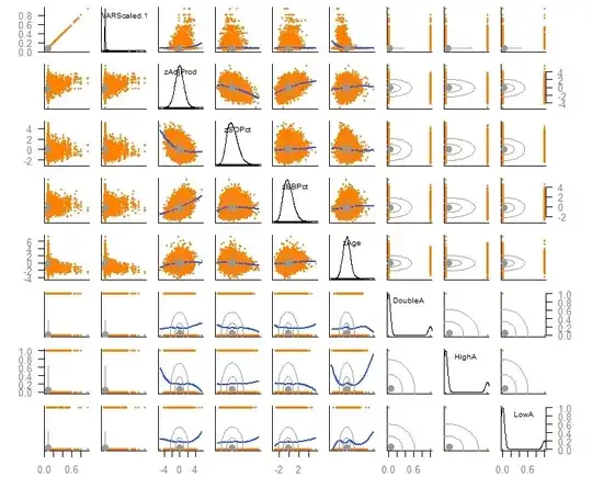
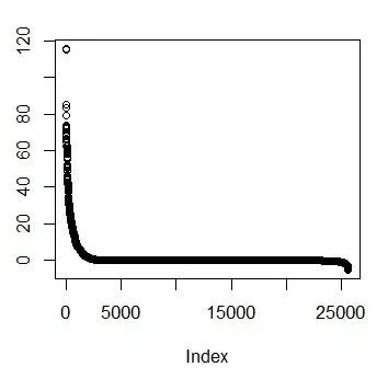
For reference, the dependent variable, oWAR, has the following plot:
I started with a linear regression oWAR = B1zAge + B2zSOPct + B3zBBPct + B4zAdjProd + B5DoubleA + B6HighA + B7LowA + B8Rookie + B9ShortSeason and obtained the following diagnostics plots:
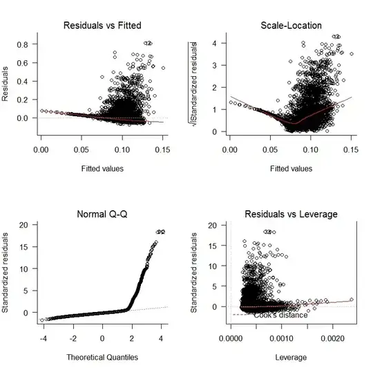
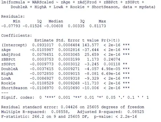
There are clear problems with a lack of unbiasedness of the residuals and a lack of random variation. Additionally, the residuals are not normal. The results of the regression are shown below:
Following the advice in a previous thread, I tried a Box-Cox transformation with no success. Next, I tried a GAM with a log link and received these plots:
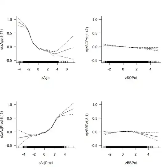
Original
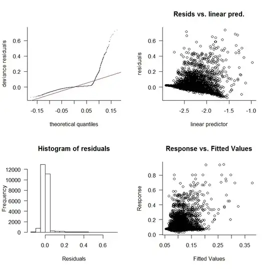
New Diagnostic Plot
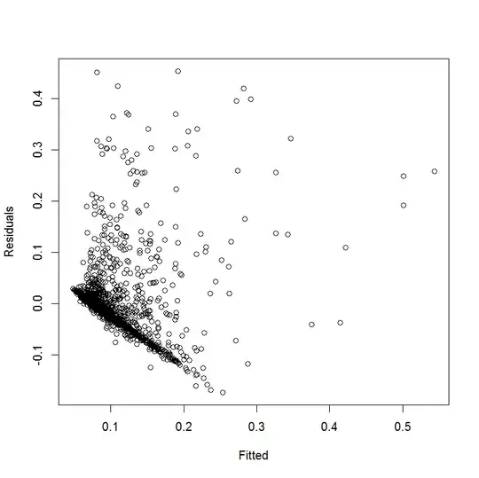
It looks like the splines helped fit the data but the diagnostic plots still show a poor fit. EDIT: I thought I was looking at the residuals vs fitted values originally but I was incorrect. The plot that was originally shown is marked as Original (above) and the plot I uploaded afterwards is marked as New Diagnostic Plot (also above)
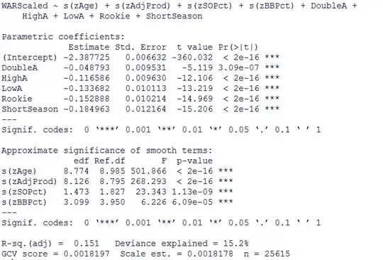
The $R^2$ of the model has increased
but the results produced by the command gam.check(myregression, k.rep = 1000) are not that promising.
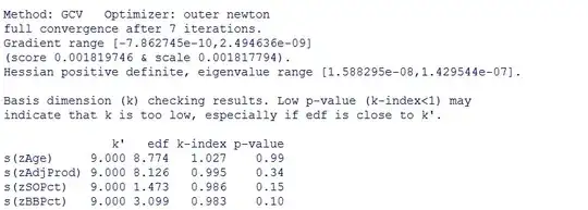
Can anyone suggest a next step for this model? I am happy to provide any other information that you think might be useful to understand the progress I've made thus far. Thanks for any help you can provide.