Removal of statistically significant intercept term increases $R^2$ in linear model

Question

In a simple linear model with a single explanatory variable,

$\alpha_i = \beta_0 + \beta_1 \delta_i + \epsilon_i$

I find that removing the intercept term improves the fit greatly (value of $R^2$ goes from 0.3 to 0.9). However, the intercept term appears to be statistically significant.

With intercept:

Call:
lm(formula = alpha ~ delta, data = cf)

Residuals:
     Min       1Q   Median       3Q      Max 
-0.72138 -0.15619 -0.03744  0.14189  0.70305 

Coefficients:
            Estimate Std. Error t value Pr(>|t|)    
(Intercept)  0.48408    0.05397    8.97   <2e-16 ***
delta        0.46112    0.04595   10.04   <2e-16 ***
---
Signif. codes:  0 ‘***’ 0.001 ‘**’ 0.01 ‘*’ 0.05 ‘.’ 0.1 ‘ ’ 1 

Residual standard error: 0.2435 on 218 degrees of freedom
Multiple R-squared: 0.316,    Adjusted R-squared: 0.3129 
F-statistic: 100.7 on 1 and 218 DF,  p-value: < 2.2e-16

Without intercept:

Call:
lm(formula = alpha ~ 0 + delta, data = cf)

Residuals:
     Min       1Q   Median       3Q      Max 
-0.92474 -0.15021  0.05114  0.21078  0.85480 

Coefficients:
      Estimate Std. Error t value Pr(>|t|)    
delta  0.85374    0.01632   52.33   <2e-16 ***
---
Signif. codes:  0 ‘***’ 0.001 ‘**’ 0.01 ‘*’ 0.05 ‘.’ 0.1 ‘ ’ 1 

Residual standard error: 0.2842 on 219 degrees of freedom
Multiple R-squared: 0.9259,   Adjusted R-squared: 0.9256 
F-statistic:  2738 on 1 and 219 DF,  p-value: < 2.2e-16

How would you interpret these results? Should an intercept term be included in the model or not?

Edit

Here's the residual sums of squares:

RSS(with intercept) = 12.92305
RSS(without intercept) = 17.69277

Answer 1

First of all, we should understand what the R software is doing when no intercept is included in the model. Recall that the usual computation of $R^2$ when an intercept is present is $$ R^2 = \frac{\sum_i (\hat y_i - \bar y)^2}{\sum_i (y_i - \bar y)^2} = 1 - \frac{\sum_i (y_i - \hat y_i)^2}{\sum_i (y_i - \bar y)^2} \>. $$ The first equality only occurs because of the inclusion of the intercept in the model even though this is probably the more popular of the two ways of writing it. The second equality actually provides the more general interpretation! This point is also address in this related question.

But, what happens if there is no intercept in the model?

Well, in that case, R (silently!) uses the modified form $$ R_0^2 = \frac{\sum_i \hat y_i^2}{\sum_i y_i^2} = 1 - \frac{\sum_i (y_i - \hat y_i)^2}{\sum_i y_i^2} \>. $$

It helps to recall what $R^2$ is trying to measure. In the former case, it is comparing your current model to the reference model that only includes an intercept (i.e., constant term). In the second case, there is no intercept, so it makes little sense to compare it to such a model. So, instead, $R_0^2$ is computed, which implicitly uses a reference model corresponding to noise only.

In what follows below, I focus on the second expression for both $R^2$ and $R_0^2$ since that expression generalizes to other contexts and it's generally more natural to think about things in terms of residuals.

But, how are they different, and when?

Let's take a brief digression into some linear algebra and see if we can figure out what is going on. First of all, let's call the fitted values from the model with intercept $\newcommand{\yhat}{\hat {\mathbf y}}\newcommand{\ytilde}{\tilde {\mathbf y}}\yhat$ and the fitted values from the model without intercept $\ytilde$.

We can rewrite the expressions for $R^2$ and $R_0^2$ as $$\newcommand{\y}{\mathbf y}\newcommand{\one}{\mathbf 1} R^2 = 1 - \frac{\|\y - \yhat\|_2^2}{\|\y - \bar y \one\|_2^2} \>, $$ and $$ R_0^2 = 1 - \frac{\|\y - \ytilde\|_2^2}{\|\y\|_2^2} \>, $$ respectively.

Now, since $\|\y\|_2^2 = \|\y - \bar y \one\|_2^2 + n \bar y^2$, then $R_0^2 > R^2$ if and only if $$ \frac{\|\y - \ytilde\|_2^2}{\|\y - \yhat\|_2^2} < 1 + \frac{\bar y^2}{\frac{1}{n}\|\y - \bar y \one\|_2^2} \> . $$

The left-hand side is greater than one since the model corresponding to $\ytilde$ is nested within that of $\yhat$. The second term on the right-hand side is the squared-mean of the responses divided by the mean square error of an intercept-only model. So, the larger the mean of the response relative to the other variation, the more "slack" we have and a greater chance of $R_0^2$ dominating $R^2$.

Notice that all the model-dependent stuff is on the left side and non-model dependent stuff is on the right.

Ok, so how do we make the ratio on the left-hand side small?

Recall that $\newcommand{\P}{\mathbf P}\ytilde = \P_0 \y$ and $\yhat = \P_1 \y$ where $\P_0$ and $\P_1$ are projection matrices corresponding to subspaces $S_0$ and $S_1$ such that $S_0 \subset S_1$.

So, in order for the ratio to be close to one, we need the subspaces $S_0$ and $S_1$ to be very similar. Now $S_0$ and $S_1$ differ only by whether $\one$ is a basis vector or not, so that means that $S_0$ had better be a subspace that already lies very close to $\one$.

In essence, that means our predictor had better have a strong mean offset itself and that this mean offset should dominate the variation of the predictor.

An example

Here we try to generate an example with an intercept explicitly in the model and which behaves close to the case in the question. Below is some simple R code to demonstrate.

set.seed(.Random.seed[1])

n <- 220
a <- 0.5
b <- 0.5
se <- 0.25

# Make sure x has a strong mean offset
x <- rnorm(n)/3 + a
y <- a + b*x + se*rnorm(x)

int.lm   <- lm(y~x)
noint.lm <- lm(y~x+0)  # Intercept be gone!

# For comparison to summary(.) output
rsq.int <- cor(y,x)^2
rsq.noint <- 1-mean((y-noint.lm$fit)^2) / mean(y^2)

This gives the following output. We begin with the model with intercept.

# Include an intercept!
> summary(int.lm)

Call:
lm(formula = y ~ x)

Residuals:
      Min        1Q    Median        3Q       Max
-0.656010 -0.161556 -0.005112  0.178008  0.621790

Coefficients:
            Estimate Std. Error t value Pr(>|t|)
(Intercept)  0.48521    0.02990   16.23   <2e-16 ***
x            0.54239    0.04929   11.00   <2e-16 ***
---
Signif. codes:  0 '***' 0.001 '**' 0.01 '*' 0.05 '.' 0.1 ' ' 1

Residual standard error: 0.2467 on 218 degrees of freedom
Multiple R-squared: 0.3571,     Adjusted R-squared: 0.3541
F-statistic: 121.1 on 1 and 218 DF,  p-value: < 2.2e-16

Then, see what happens when we exclude the intercept.

# No intercept!
> summary(noint.lm)

Call:
lm(formula = y ~ x + 0)

Residuals:
     Min       1Q   Median       3Q      Max
-0.62108 -0.08006  0.16295  0.38258  1.02485

Coefficients:
  Estimate Std. Error t value Pr(>|t|)
x  1.20712    0.04066   29.69   <2e-16 ***
---
Signif. codes:  0 '***' 0.001 '**' 0.01 '*' 0.05 '.' 0.1 ' ' 1

Residual standard error: 0.3658 on 219 degrees of freedom
Multiple R-squared: 0.801,      Adjusted R-squared: 0.8001
F-statistic: 881.5 on 1 and 219 DF,  p-value: < 2.2e-16

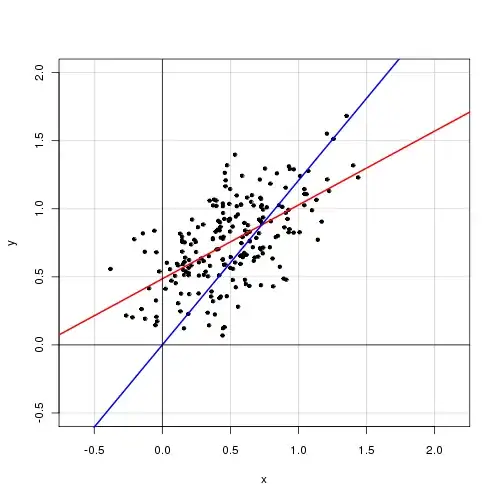
Below is a plot of the data with the model-with-intercept in red and the model-without-intercept in blue.

Answer 2

I would base my decision on an information criteria such as the Akaike or Bayes-Schwarz criteria rather than R^2; even then I would not view these as absolute.

If you have a process where the slope is near zero and all of the data is far from the origin, your correct R^2 should be low as most of the variation in the data will be due to noise. If you try to fit such data to a model without an intercept you will generate a large and wrong slope term and likely a better looking R^2 if the intercept free version is used.

The following graph shows what happens in this extreme cases. Here the generating process is that x=100,100.1,.... and y is just 100 + random noise with mean 0 and standard deviation .1. The points are black circles, the fit without the intercept is the blue line and the fit with the intercept (zeroing out the slope) is the red line:

[Sorry it won't let me post the graph; run the R-code below to generate it. It shows the origin in the lower left corner, the cluster of points in the upper right corner. The bad no-intercept fit goes from the lower left to the upper right and the correct fit is a line parallel to the x-axis]

The correct model for this should have an R^2 of zero---be a constant plus random noise. R will give you and R^2 of .99 for the fit with no intercept. This won't matter much if you only use the model for prediction with x-values within the range of the training data, but will fail miserably if x goes outside of the narrow range of the training set or you are trying to gain true insights beyond just prediction.

The AIC correctly shows that the model with the intercept is preferred. The R code for this is:

 Nsamp=100
x=seq(1,100,1)*.1+100 # x=101.1,101.2,....
y=rnorm(n=length(x))+100 # random noise +100 (best model is constant)

model_withint=lm(y~x)
print(summary(model_withint))
flush.console()
model_noint=lm(y~x+0) 
print(summary(model_noint))
print (AIC(model_withint))
print(sprintf ('without intercept  AIC=%f',AIC(model_noint)))
print(sprintf ('with intercept  AIC=%f',AIC(model_withint)))
print(sprintf ('constant model  AIC=%f',AIC(lm(y~1))))
plot(x,y,ylim=c(0,105),xlim=c(0,105))
lines( c(0,105),c(0,105)*model_noint$coefficients['x'],col=c('blue'))
lines( c(0,105),c(1,1)*(lm(y~1)$coefficients['(Intercept)']),col=c('red'))

The AIC output is

   "without intercept  AIC=513.549626"
    "with intercept  AIC=288.112573"
    "constant model  AIC=289.411682"

Note that the AIC still gets the wrong model in this case, as the true model is the constant model; but other random numbers will yield data for which the AIC is lowest for the constant model. Note that if you discard the slope, you should refit the model without it, not try to use the intercept from the model and ignore the slope.