64

The coefficient of an explanatory variable in a multiple regression tells us the relationship of that explanatory variable with the dependent variable. All this, while 'controlling' for the other explanatory variables.

How I have viewed it so far:

While each coefficient is being calculated, the other variables are not taken into account, so I consider them to be ignored.

So am I right when I think that the terms 'controlled' and 'ignored' can be used interchangeably?

Siddharth Gopi
  • 1,395
  • 1
  • 12
  • 22
  • 2
    I wasn't so enthused about this question until I saw the two figured you inspired @gung to offer. – DWin Dec 07 '13 at 04:22
  • 1
    You weren't aware of the conversation we were having elsewhere that motivated this question, @DWin. It was too much to try to explain this in a comment, so I asked the OP to make it a formal question. I actually think explicitly bringing out the distinction b/t ignoring & controlling for other variables in regression is a great question, & I glad it got discussed here. – gung - Reinstate Monica Dec 07 '13 at 04:27
  • 2
    see also the first diagram [here](http://en.wikipedia.org/wiki/Simpson%27s_paradox) – Glen_b Dec 07 '13 at 09:30
  • 1
    Is the data used in this question available so we could run it ourselves as a educating sample. – Larry Aug 23 '17 at 03:56

2 Answers2

105

Controlling for something and ignoring something are not the same thing. Let's consider a universe in which only 3 variables exist: $Y$, $X_1$, and $X_2$. We want to build a regression model that predicts $Y$, and we are especially interested in its relationship with $X_1$. There are two basic possibilities.

  1. We could assess the relationship between $X_1$ and $Y$ while controlling for $X_2$:
    $$ Y = \beta_0 + \beta_1X_1 + \beta_2X_2 $$ or,
  2. we could assess the relationship between $X_1$ and $Y$ while ignoring $X_2$:

    $$ Y = \beta_0 + \beta_1X_1 $$

Granted, these are very simple models, but they constitute different ways of looking at how the relationship between $X_1$ and $Y$ manifests. Often, the estimated $\hat\beta_1$s might be similar in both models, but they can be quite different. What is most important in determining how different they are is the relationship (or lack thereof) between $X_1$ and $X_2$. Consider this figure:

enter image description here

In this scenario, $X_1$ is correlated with $X_2$. Since the plot is two-dimensional, it sort of ignores $X_2$ (perhaps ironically), so I have indicated the values of $X_2$ for each point with distinct symbols and colors (the pseudo-3D plot below provides another way to try to display the structure of the data). If we fit a regression model that ignored $X_2$, we would get the solid black regression line. If we fit a model that controlled for $X_2$, we would get a regression plane, which is again hard to plot, so I have plotted three slices through that plane where $X_2=1$, $X_2=2$, and $X_2=3$. Thus, we have the lines that show the relationship between $X_1$ and $Y$ that hold when we control for $X_2$. Of note, we see that controlling for $X_2$ does not yield a single line, but a set of lines.

enter image description here

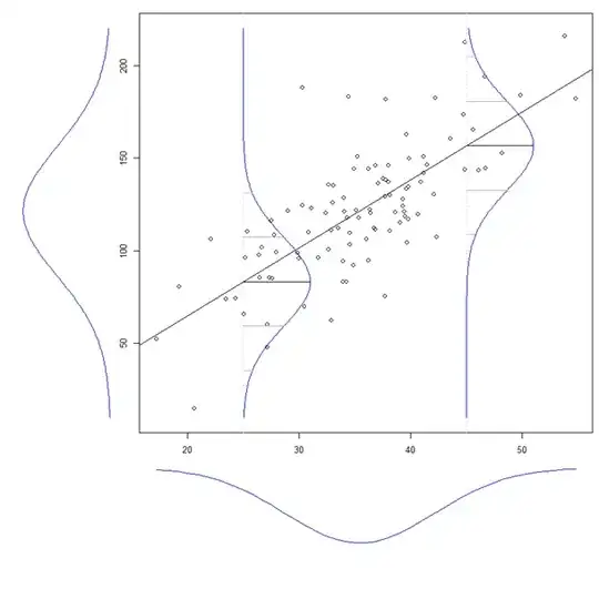
Another way to think about the distinction between ignoring and controlling for another variable, is to consider the distinction between a marginal distribution and a conditional distribution. Consider this figure:

enter image description here

(This is taken from my answer here: What is the intuition behind conditional Gaussian distributions?)

If you look at the normal curve drawn to the left of the main figure, that is the marginal distribution of $Y$. It is the distribution of $Y$ if we ignore its relationship with $X$. Within the main figure, there are two normal curves representing conditional distributions of $Y$ when $X_1 = 25$ and $X_1 = 45$. The conditional distributions control for the level of $X_1$, whereas the marginal distribution ignores it.

gung - Reinstate Monica
  • 132,789
  • 81
  • 357
  • 650
  • 2
    Gung, this is enlightening, I am glad I made the mistake of using the word 'ignore' in my answer to that question. Im now going to try find out how exactly statistical packages 'control' for the other variables. (My first thought is they use some measure like the pearson correlation coefficient. With many explanatory variables, things would get messy though) Thank you for this answer! – Siddharth Gopi Dec 07 '13 at 02:50
  • 1
    You're welcome, @garciaj, although I'm not done yet ;-). I'm looking for another figure; I may have to make it from scratch. – gung - Reinstate Monica Dec 07 '13 at 02:52
  • I added the last part, @garciaj, although you may already understand the idea at this point. Regarding how it's done, it simply falls out of the math of finding estimated slopes that minimize the OLS loss function (cf my [comment](http://stats.stackexchange.com/questions/71260//71262#comment138162_71262) at the linked answer &/or my answer [here](http://stats.stackexchange.com/questions/22718//22721#22721)). For an intuition, you could think of each variable but 1 being held at their means & then the slope of the remaining variable is found (at least when there are no interactions). – gung - Reinstate Monica Dec 07 '13 at 03:56
  • You illustrate a critical point. The "reversal", i.e. change of sign, of an estimated effect conditional on a regressor is not something that is often handled well, but your new illustration makes it very clear how that result might occur. – DWin Dec 07 '13 at 04:20
  • Thanks, @DWin. I actually have (essentially) that figure in some other answer somewhere, but I couldn't find it, nor could I find the code file I had used to make it, so I had to remake it from scratch. I have more ways of trying to explain conditional vs. marginal, but this should be enough. – gung - Reinstate Monica Dec 07 '13 at 04:22
  • The graphical demonstration is very valuable. It keeps the reality of the data (and the fact that it was obtained from a sampling process) in better focus. – DWin Dec 07 '13 at 04:25
  • 4
    The crucial idea in the first figure is that those points lie in a three-dimensional space, w/ the red circles on a flat plane at the computer screen, the blue triangles on a parallel plane a little in front of the screen & the green pluses on a plane a little in front of that. The regression plane tilts downward to the right, but slopes upward as it moves out from the screen towards you. Note that this phenomenon occurs because X1 & X2 are correlated, if they were uncorrelated, the estimated betas would be the same. – gung - Reinstate Monica Dec 07 '13 at 14:52
  • @gung In the first graph, is the slope of the regression line when controlling $X_2$ the same for every value of $X_2$? I'm just trying to tie this back to my [all else equal](http://stats.stackexchange.com/questions/84314/what-does-all-else-equal-mean-in-multiple-regression) post. – EconStats Feb 04 '14 at 00:39
  • @EconStats, there is no interaction here, or other variable that is a function of $X_1$, so the slope of the regression line controlling for $X_2$ is the same at every value of $X_2$. – gung - Reinstate Monica Feb 04 '14 at 00:56
  • @gung amazing explaining done here. Truly! A small follow-up question: I am just curious as to how the estimation is actually done. Regarding your first plot, we have three OLS lines, each giving us a value for $\beta_1$. What happens if these three values of $\beta_1$ are different? Do one just take an average of the three estimated $beta_1$'s? I feel it is hard to think about how to understand what happens in the estimation and connecting this to the actual ols estimation $\beta=(X^TX)^{-1}X^Ty$ – Erosennin Apr 16 '15 at 07:55
  • @ErosRam, that might be better as a new question. Briefly, when you have 2 X variables, you are fitting a plane instead of a line. If the appropriate slope of the y~x2 relationship changes as x1 increases, that means there is an interaction b/t x1&x2. – gung - Reinstate Monica Apr 16 '15 at 16:31
  • Thank you @gung. I made a new question, as you suggested, trying to sum up all my thoughts and questions. I hope you don't mind I borrowed one of your plots from this post. If you do, I will of course remove it right away. Here is a link to my question: http://stats.stackexchange.com/questions/146859/estimation-process-in-ols-with-categorical-variables-and-dummy-coding – Erosennin Apr 17 '15 at 08:10
  • 1
    And this kind of correlation among predictors (e.g., @gung scenario) is what usually underlies a case of [the Simpson's paradox](https://en.wikipedia.org/wiki/Simpson%27s_paradox#Correlation_between_variables). In a universe with more than three variables, it is wise to remember that it may be lurking your inferences (d'oh!). – FairMiles Apr 19 '16 at 15:03
  • @gung :Sorry for the necropost. IS it accurate to say that controlling for a variable X is equivalent to fixing the value of X? Example: if we control salary for years of education, aren't we regressing over all people with the same amount of education, e.g., we hold the years of education constant? – MSIS Aug 20 '16 at 21:52
  • 2
    @MSIS, when you control for a variable in a model, the model tries to hold it constant (fixed) for the sake of estimating everything else in the model. However, this is just an attempt & subject to random error, so it isn't necessarily identical to what you would get if you ran a study w/ a variable physically fixed at a given value. – gung - Reinstate Monica Aug 21 '16 at 14:18
  • @gung: thank you, just to double check. say I wanted to control for income X1 in Y=a1X1+a2X2+a3X3 , for, say , people making $40,000. Would my regression equation become Y=a140,000+a2X2+a3X3, I guess a conditional regression, a sort of "slice"? This would then lower the dimension by 1? Sorry if I am being thick here, and thanks again. – MSIS Aug 22 '16 at 15:31
  • I'm not sure I follow you, @MSIS. It might be better to ask a new question than try to hash this out in comments. If you wanted to have income fixed, you would only gather data on people who make exactly $40k, & then not include income in the model to be fitted. – gung - Reinstate Monica Aug 22 '16 at 15:59
  • This is a great answer, @gung! I love the graphs! Albeit we can "see" the estimates for X1 and X2 in the first graph, maybe adding them as numbes as well in the text below the graph emphasises a bit how they change in the two settings? – Helix123 Oct 24 '17 at 08:48
  • Dear gung, can we say controlling for another predictor means what I mention [HERE](https://stats.stackexchange.com/questions/483172/holding-other-predictors-constant-via-simulation-in-r)? – rnorouzian Aug 16 '20 at 04:45
9

They are not ignored. If they were 'ignored' they would not be in the model. The estimate of the explanatory variable of interest is conditional on the other variables. The estimate is formed "in the context of" or "allowing for the impact of" the other variables in the model.

DWin
  • 7,005
  • 17
  • 32
  • The estimate is of course subject to other variables. But we must purify it by introducing the so-called other factors in the model. However, sometimes these factors may be of categorical nature and cause more problems than give a valid solution. –  Dec 25 '13 at 10:08
  • That's certainly true and it doesn't arise just for categorical variables. Continuous and ordinal variables can cause invalid inferences if the underlying science and reality are not taken into account properly, – DWin Mar 03 '21 at 23:44