Adding a quadratic term flips the signs of the coefficients

Question

So I have a question of utilizing quadratic (second order) predictors with GLMs in R. Basically I have three predictor variables $(x, y, z)$ and a response variable (let's call it ozone). $x$, $y$, and $z$ are not inherently quadratic predictors yet so I square them (X2 <- x^2, and likewise for y and z).

Now I understand that if I wanted to model ozone based on these predictor variables I would use the poly() or polym() function (to create orthogonal polynomials).

However, when it comes to using interaction terms between these three variables, that's where I get lost. For example, if I wanted to model the interaction between the quadratic predictors of $x$ and $y$ I believe I would be typing in something like this

ozone <- x + y+ x^2 + y^2+ xy + x^2y + xy^2 + x^2y^2  # (I hope this is right)

My questions are:

1. Is there an easier way of inputting this (with three terms that's a lot of typing).
2. Why does the quadratic predictor flip signs of the coefficients? When I just run the predictor variable $x$ the coefficient is positive but when I use a quadratic predictor the coefficient almost always ends up being negative.

If you follow this link, it'll show you my initial question on Stack Overflow. In terms of the context of this question (which was non existent in the initial post), it's based on a dataframe consisting of predictor variables of radiation, temperature, and wind and the response variable of ozone levels in the atmosphere. Therefore, x, y, and z in the initial post were those three predictors.

Ultimately, are the statistical solutions given by others in that post valid?

Answer 1

This is a Q&A site for questions about statistics, not for questions about how R works or how to use it. Your question #1 is off topic here, and I don't see why you want us to say if what they told you on Stack Overflow was correct—that is the appropriate site for R coding questions. At any rate, you can get the canonical answer in the documentation for formulae for statistical models in the Intro to R manual:

y ~ poly(x,2)
...
         Polynomial regression of y on x of degree 2. ...

...
y ~ A*B
y ~ A + B + A:B
...
         Two factor non-additive model of y on A and B. ...

From these you can see that you can get an interaction between two polynomials like so:

poly(x,2)*poly(y,2)

---

Regarding your question about the sign changing, there are several ways to think about this. First of all, when you add another variable, the signs of existing variables can change (see: here, and here, e.g.), and from the model's perspective, a squared term is just another variable (see: Why is polynomial regression considered a special case of multiple linear regression?). On the other hand, I have argued that we should consider all polynomial terms together when interpreting a model (cf., Does it make sense to add a quadratic term but not the linear term to a model?). Still, it may seem weird to think that the squared term is correlated with the original variable, and it is legitimate to wonder what that means.

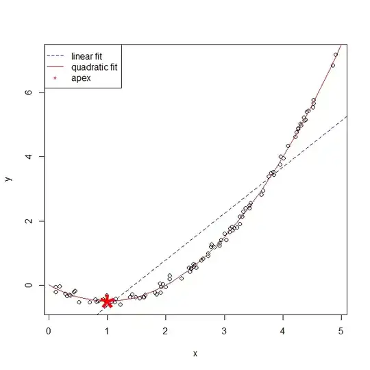
For what it's worth, if you use poly(x,2), you will get orthogonal polynomials and there won't be an issue; likewise if you center your x variable before squaring, cf., here. However, the issue remains if you simply square your x variable in the most intuitive way (as you did), or use poly(x, 2, raw=TRUE). So, what does it mean for the coefficient on x to become, say, negative where it was positive before? As @whuber explains in his answer here, when you have (only) an $x$ and an $x^2$ term, you will have a parabola, and the x-value of the location of the apex of the parabola will be related to those coefficients. More specifically, if we call the coefficients on $x$ and $x^2$ $\beta_1$ and $\beta_2$ (eliding the hats for simplicity), the x position of the apex is $\beta_1/-2\beta_2$. (This is complicated, because it is also contingent on the value of $\beta_2$. Moreover, $\beta_2$ will be positive when the parabola is concave up—and vice versa; without loss of generality, let's assume that is your case.) So here a negative value of $\beta_1$ makes the x location of the apex to the right of $0$. You can see this demonstrated in the example below (coded in R):

set.seed(981)                 # this makes the example exactly reproducible
x = runif(100, min=0, max=5)  # here I generate some data
y = 0 -1*x + .5*x**2 + rnorm(100, mean=0, sd=.1)

m.l = lm(y~x)                 # here I fit linear & quadratic models
m.p = lm(y~poly(x, 2, raw=TRUE))
summary(m.l)$coefficient      # these are the fitted coefficients:
#              Estimate Std. Error   t value     Pr(>|t|)
# (Intercept) -2.103753 0.18623242 -11.29639 1.911436e-19
# x            1.445807 0.06430754  22.48270 1.822846e-40
summary(m.p)$coefficient
#                             Estimate Std. Error     t value     Pr(>|t|)
# (Intercept)              0.009625853 0.02979478   0.3230718 7.473363e-01
# poly(x, 2, raw = TRUE)1 -1.008168121 0.02698804 -37.3561142 2.216150e-59
# poly(x, 2, raw = TRUE)2  0.501424686 0.00533965  93.9059119 4.859026e-97

xs   = seq(0,5, by=.1)        # this code makes the plot
apex = coef(m.p)[2] / (-2*coef(m.p)[3])
windows()
  plot(x, y)
  abline(coef(m.l), col="blue", lty=2)
  lines(xs, predict(m.p, data.frame(x=xs)), col="red")
  points(apex, predict(m.p, data.frame(x=apex)), col="red", pch="*", cex=5)
  legend("topleft", legend=c("linear fit", "quadratic fit", "apex"),
         lty=c(2,1,NA), pch=c(NA, NA, "*"), col=c("blue","red","red"))