7

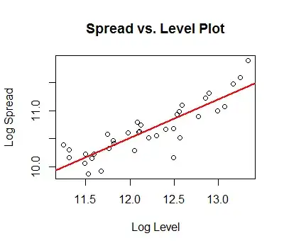
With the below dataset, I have a series which needs transforming. Easy enough. However, how do you decide which of the SQRT or LOG transformations is better? And how do you draw that conclusion?

x<-c(75800,54700,85000,74600,103900,82000,77000,103600,62900,60700,58800,134800,81200,47700,76200,81900,95400,85400,84400,103400,63000,65500,59200,128000,74400,57100,75600,88300,111100,95000,91500,111400,73700,72800,64900,146300,83100,66200,101700,100100,120100,100200,97000,120600,88400,83500,73200,141800,87700,82700,106000,103900,121000,98800,96900,115400,87500,86500,81800,135300,88900,77100,109000,104000,113000,99000,104500,109400,92900,88700,90500,140200,91700,78800,114700,100700,113300,122800,117900,122200,102900,85300,92800,143800,88400,75400,111200,96300,114600,108300,113400,116600,103400,87300,88200,149800,90100,78800,108900,126300,122000,125100,119600,148800,114600,101600,108800,174100,101100,89900,126800,126400,141400,144700,132800,149000,124200,101500,106100,168100,104200,79900,126100,121600,139500,143100,144100,154500,129500,109800,116200,171100,106700,85500,132500,133700,135600,149400,157700,144500,165400,122700,113700,175000,113200,94400,138600,132400,129200,165700,153300,141900,170300,127800,124100,206700,131700,112700,170900,153000,146700,197800,173800,165400,201700,147000,144200,244900,146700,124400,168600,193400,167900,209800,198400,184300,214300,156200,154900,251200,127900,125100,171500,167000,163900,200900,188900,168000,203100,169800,171900,241300,141400,140600,172200,192900,178700,204600,222900,179900,229900,173100,174600,265400,147600,140800,171900,189900,185100,218400,207100,178800,228800,176900,170300,251500,149900,150300,192000,185100,184500,228800,219000,180000,241500,184300,174600,264500,166100,151900,194600,214600,201700,229400,233600,197500,254600,194000,201100,279500,175800,167200,235900,207400,215900,261800,236800,222400,281500,214100,218200,295000,194400,180200,250400,212700,251300,280200,249300,240000,304200,236900,232500,300700,207300,196900,246600,262500,272800,282300,271100,265600,313500,268000,256500,318100,232700,198500,268900,244300,262400,289200,286600,281100,330700,262000,244300,309300,246900,211800,263100,307700,284900,303800,296900,290400,356200,283700,274500,378300,263100,226900,283800,299900,296000,327600,313500,291700,333000,246500,227400,333200,239500,218600,283500,267900,294500,318600,318700,283400,351600,268400,251100,365100,249100,216400,245500,232100,236300,275600,296500,296900,354300,277900,287200,420200,299700,268200,329700,353600,356200,396500,379500,349100,437900,350600,338600,509100,342300,288800,378400,371200,395800,450000,414100,387600,486600,355300,358800,526800,346300,295600,361500,415300,402900,484100,412700,395800,491300,391000,374900,569200,369500,314900,422500,436400,439700,509200,461700,449500,560600,435000,429900,633400,417900,365700,459200,466500,488500,531500,483500,485400,575700,458000,433500,642600,409600,363100,430100,503900,500400,557400,565500,526700,628900,547700,520400,731200,494400,416800,558700,537100,556200,686700,616600,582600,725800,577700,552100,806700,554200,455000,532600,693000,619400,727100,684700)
y<-ts(x,frequency=12, start=c(1976,1))
#Transforming the data to log or sqrt and plotting it
log.y<-log(y)
plot(log.y)
sqrt.y<-sqrt(y)
plot(sqrt.y)
cardinal
  • 24,973
  • 8
  • 94
  • 128
digdeep
  • 195
  • 2
  • 2
  • 7
  • Log if that's the choice. Behaviour looks much simpler on log scale, trend is more nearly linear and variability about constant. But a Poisson regression might do just as well without the transforming-back-transforming stuff so long as you think about serial dependence. That's heresy for those who incline to the view "time series require time series software, period". – Nick Cox Nov 04 '13 at 13:48
  • @NickCox Solutions shouldn't be less than they should be or more than they should be. If you have time series data then the analysis (probably) requires time series software as simple solutions often lead to simply incorrect conclusions. Here I stand , I can do no other ... said a favorite heretic of mine. – IrishStat Nov 04 '13 at 22:42
  • There are many examples of models fitted to data in time that are not time series models, e.g. growth models. At first blush this model looks well fitted by an exponential plus sinusoidal terms. If so, I would not push it into a Box-Jenkins-type ARIMA plus bells and whistles mode. Unfortunately, there is no substantive context in this question to guide recommendations. – Nick Cox Nov 04 '13 at 23:47
  • @NickCox validation of the Gaussian assumptions are not bells and whistles but the underpining of the GLM. – IrishStat Nov 05 '13 at 00:36
  • 1
    I am alluding to your extra machinery for "Level Shifts, Seasonal Pulses and/or Local Time Trends". – Nick Cox Nov 05 '13 at 00:39
  • @Nick These are schemes for pulling non-random structure out of the residuals and rendering it free of both stochastic and deterministic structure. These are definitely not bells and whistles just because they don't appear in some software offerings. – IrishStat Nov 05 '13 at 00:55
  • I understand your broad intention here. "Bells and whistles" is not pejorative in my language; it just refers to secondary features in addition to whatever captures trend and seasonality. – Nick Cox Nov 05 '13 at 00:59
  • The devil is in the details. There are no secondary features just a seamless integration/identification of significant features. Ignoring some features con lead to misidentification of other features such as the ignoring of outliers can lead to misidentification of supposedly needed power transformations. It is not widely known but the Box-Cox test premises no anomalies. Please see http://www.autobox.com/pdfs/vegas_ibf_09a.pdf for a discussion about the classic Airline Series from Box and Jenkins. – IrishStat Nov 05 '13 at 12:05
  • Thank you both for the detailed info, wish i had a chance earlier to log in. @NickCox hope this is further context re previous post. The dataset is airline passenger monthly short term arrivals. Dataset is really just something to learn from. The basis for my post was to truly understand why you would take a specific transformation option over the other to then fit SARIMA(p,d,q)(P,D,Q)12 model. Actually, trying to replicate this for SAS (pretty new to SAS) I thought if I can see it in R I can transfer my knowledge of R and replicate it using SAS as I am trying to learn the language. – digdeep Nov 05 '13 at 13:02
  • @IrishStat We are applying different vocabulary to the same enterprise. I look at this series and I see trend (massive) and seasonality (clear). The question then is what else might there be as well. I call those secondary features. Your procedures find various other details and build them into your model. I suspect that many data analysts would (a) prefer more parsimonious models to yours (b) wonder about how many parameters you are estimating and how many preliminary significance tests go into your model choice. These questions range from style preferences to important technicalities. – Nick Cox Nov 05 '13 at 13:52
  • @Nick with 427 values , the number of parameters(12) in my final model is hardly a consideration. What is very true is the notion of "many t tests" but this is an aspect of search procedures which speak to augmentation while limiting the scope of that augmentation. Evaluating opportunities (the model sample space) has to be done carefully and in a way that doesn't overfit but sufficiently fits. – IrishStat Nov 05 '13 at 16:06

3 Answers3

15

This question is answered beautifully by means of a spread-versus-level plot: a cube root transformation will stabilize the spreads of the data, providing a useful basis for further exploration and analysis.


The data show a clear seasonality:

plot(y)

Data

Take advantage of this by slicing the data into annual (or possibly biennial) groups. Within each group compute resistant descriptors of their typical value and their spread. Good choices are based on the 5-letter summary, consisting of the median (which splits the data into upper and lower halves), the medians of the two halves (the "hinges" or "fourths"), and the extremes. Because the extremes are not resistant to outliers, use the difference of the hinges to represent the spread. (This "fourth-spread" is the length of a box in a properly constructed box-and-whisker plot.)

spread <- function(x) {
  n <- length(x)
  n.med <- (n + 1)/2
  n.fourth <- (floor(n.med) + 1)/2
  y <- sort(x)[c(floor(n.fourth), ceiling(n.fourth), 
               floor(n+1 - n.fourth), ceiling(n+1 - n.fourth))]
  return( y %*% c(-1,-1,1,1)/2 )
}
years <- floor((1:length(x) - 1) / 12)
z <- split(x, years)
boxplot(z, names=(min(years):max(years))+1976, ylab="y")

Raw boxplots

The boxplots clearly get longer over time as the level of the data rises. This heteroscedasticity complicates analyses and interpretations. Often a power transformation can reduce or remove the heteroscedasticity altogether.

A spread versus level plot shows whether a power transformation (which includes the logarithm) will be helpful for stabilizing the spread within the groups and suggests an appropriate value for the power: it is directly related to the slope of the spread-vs.-level plot on log-log scales.

z.med <- unlist(lapply(z, median))
z.spread <- unlist(lapply(z, spread))
fit <- lm(log(z.spread) ~ log(z.med))
plot(log(z.med), log(z.spread), xlab="Log Level", ylab="Log Spread", 
     main="Spread vs. Level Plot")
abline(fit, lwd=2, col="Red")

Spread vs level plot

This plot shows good linearity and no large outliers, attesting to a fairly regular relationship between spread and level throughout the time period.

When the fitted slope is $p$, the power to use is $\lambda=1-p$. Upon applying the suggested power transformation, the spread is (approximately) constant regardless of the level (and therefore regardless of the year):

lambda <- 1 - coef(fit)[2]
boxplot(lapply(z, function(u) u^lambda), names=(min(years):max(years))+1976, 
        ylab=paste("y^", round(lambda, 2), sep=""),
        main="Boxplots of Re-expressed Values")

Boxplots of re-expressed values

plot(y^lambda, main= "Re-expressed Values", ylab=paste("y^", round(lambda, 2), sep=""))

Plot of re-expressed values

Often, powers that are reciprocals of small integers have useful or natural interpretations. Here, $\lambda = 0.32$ is so close to $1/3$ that it may as well be the cube root. In practice, one might choose to use the cube root, or perhaps round it to the even simpler fraction $1/2$ and take the square root, or sometimes go all the way to the logarithm (which corresponds to $\lambda = 0$).


Conclusions

In this example, the spread-versus-level plot (by virtue of its approximate linearity and lack of outliers) has shown that a power transformation will effectively stabilize the spread of the data and has automatically suggested the power to use. Although powers can be computed using various methods, none of the standard methods provides the insight or diagnostic power afforded by the spread-versus-level plot. This should be in the toolkit of every data analyst.


References

Tukey, John W. Exploratory Data Analysis. Addison-Wesley, 1977.

Hoaglin, David C., Frederick Mosteller, and John W. Tukey, Understanding Robust and Exploratory Data Analysis. John Wiley and Sons, 1983.

whuber
  • 281,159
  • 54
  • 637
  • 1,101
  • 3
    This is very nicely done as always. I would put a bit more emphasis on getting trend right first and a bit less on getting the handling of variability. That boosts the case for logarithms. No bias against cube roots, which feature in various papers of mine. – Nick Cox Nov 04 '13 at 23:47
  • 1
    @whuber thanks for the detailed write up. Really helpful post and some neat R code too. – digdeep Nov 05 '13 at 13:09
  • 1
    @Nick I agree that the trends (pre-2004 and post-2004 separately) are more linear for the logs. Some method to handle the heteroscedasticity would be essential for making forecasts: without that, forecasts based on the untransformed data would have optimistically narrow prediction intervals whereas forecasts based on logs would have pessimistically wide intervals. A short-term forecast may be robust to deviations from linearity--making cube roots a good first choice--but making longer-term forecasts does require close attention to the trend, initially favoring the log as you claim. – whuber Nov 05 '13 at 18:27
  • @whuber I did power transformation on a ts and got -0.870478 as value of lambda (since slope > 1). After applying it, the *trend is reversed* - Is this (negative power and trend reversal) okay while stabilizing the variance? – StatsMonkey Jul 22 '20 at 14:10
  • 1
    @Stats It's ok, but one of the virtues of the Box-Cox transformation (instead of the straight power transformation) is that it does not reverse trends. The Box-Cox analog of your transformation is $x\to (x^{-0.87}-1)/(-0.87).$ Notice how the division by the (negative) power reverses the trend back again. See https://stats.stackexchange.com/a/467525/919 for more discussion. – whuber Jul 22 '20 at 14:48
9

Transformations are like drugs ! Some are good for you and some aren't !. Haphazard selection of transformations should be studiously avoided.

a) One of the requirements in order to perform valid statistical tests of necessity is that the variance of the errors from the proposed model must not be proven to be non-constant. If the variance of the errors changes at discrete points in time then one has recourse to Generalized Least Squares or GLM .

b) If the variance of the errors is linearly relatable to the level of the observed series then a Logarithmic Transformation might be appropriate. If the square root of the variance of the errors is linearly relatable to the level of the original series then a Square Root transformation is appropriate. More generally the appropriate power transformation is found via the Box-Cox test where the optimal lambda is found. Note that the Box-Cox test is universally applicable and doesn't soley requite time series or spatail data.

All of the above ( a and b ) require that the mean of the errors cannot be proven to differ significantly from zero for all points. If your data is not time series or spatial in nature then the only anomaly you can detect is a pulse. However if your data is time series or spatial then Level Shifts , Seasonal Pulses and/or Local Time Trends might be suggested to render the mean value of the error term to be 0.0 everywhere or at least not significantly different from 0.0 .

In my opinion one should never willy-nilly transform the data unless one has to in order to satisfy (in part) the Gaussian assumptions. Some econometricians take logs for the simple and simply wrong reason in order to obtain direct estimates of elasticity's rather than assessing the % change in Y for a % change in x from the best model.

Now one caveat, if one knows from theory or at least one thinks that one knows from theory that transformations are necessary i.e. proven by previous well-documented research , then by all means follow that paradigm as it may prove to be more beneficial that the empirical procedures I have laid out here.

In closing use the original data, minimize any warping of the results by mindless transformations, test all assumptions and sleep well at night. Statisticians like Doctors should never do harm to their data/patients y providing drugs/transformations that have nasty and unwarranted side-effects.

Hope This Helps .

Data Analysis using time series techniques on time series data:

a plot enter image description here suggests a series that has structural change. The Chow Test yielded a signifciant break point
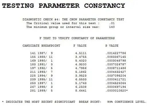
 enter image description here . enter image description here . Analysis of the modt recent 147 values starting at 1999/5 yielded enter image description here 
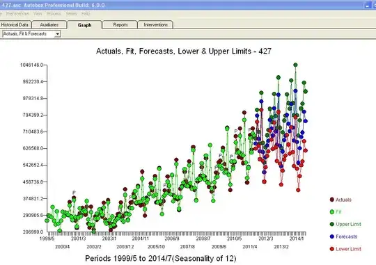
with a Residual Plot enter image description here 
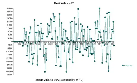
with the following ACF enter image description here . The forecast plot is enter image description here 
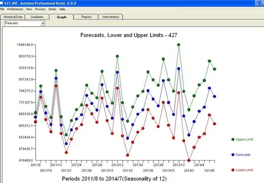
. The final model is enter image description here 
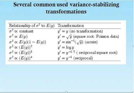
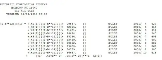
with all parameters statistically significant and no unwarranted power transformations which often unfortunately lead to wildly explosive and unrealistic forecasts. Power transforms are justified whrn it is proven via a Box-Cox test that the variablility of the ERRORS is related to the expected value as detailed here. N.B. that the variability of the original series is not used but the variability of model errors.

enter image description here

IrishStat
  • 27,906
  • 5
  • 29
  • 55
4

@digdeep, as usual @whuber provided an excellent and comprehensive answer from a statistical view point. I'm not trained in statistics, so take this response with a grain of salt. I have used the response below in my real world practice data, so I hope this is helpful.

I'll try to provide a non statistician view of transformation of time series data for Arima modeling. There is no straightforward answer. Since you are interested in knowing which transformation to use, it might be helpful to review why we do transformation.We do transformation for 3 main reasons and there might be ton of other reasons:

  1. Transformation makes the data's linear structure more usable for
    ARIMA modeling.
  2. If variance in the data is increasing or changing then transformation of data might be helpful to stabilize the variance in data.
  3. Transformation also makes the errors/residuals in ARIMA model normally distributed which is a requirement in ARIMA modeling proposed by Box-Jenkins.

There are several data transformations including Box-Cox, Log, square root, quartic and inverse and other transformations mentioned @irishstat. As with all the statistical methods there is no good guidance/answer on which transformation to select for a particular dataset.

As the famous statistician G.E.P Box said "All models are wrong but some are useful", this would apply to the transformations as well "All transformations are wrong but some are useful".

The best way to choose a transformation is to experiment. Since you have a long time series, I would hold out the last 12 - 24 months, and build a model using all the transformation and see if a particular transformation is helpful at predicting your out of sample data accurately. Also examine the residuals for normality assumption of your model. Hopefully, this would guide you in choosing an appropriate transformation. You might also want to compare this with non-transformed data and see if the transformation helped your model.

@whuber's excellent graphical representation of your data motivated me to explore this data graphically using a decomposition method. I might add, R has an excellent decomposition method called STL which would be helpful in identifying patterns that you would normally not notice. For a dataset like this, STL decomposition is helpful in not only selecting an appropriate method for analyzing your data, it might also be helpful in identifying anomalies such as outliers/level shift/change in seasonality etc., See below. Notice that the remainder (irregular) component of the data, looks like there is stochastic seasonality and the variation is not random, there appears to be a pattern. See also change in level of trend component after 2004/2005 that @whuber is refrencing.

Hopefully this is helpful.

g <- stl(y,s.window = "periodic")
plot(g)

enter image description here

forecaster
  • 7,349
  • 9
  • 43
  • 81