In general this is such a nasty problem that we shouldn't apply automatic optimizers like nls in R. However, it is easily solvable upon observing that the model is linear, and meets the assumptions of ordinary least squares (OLS) estimation, conditional upon the value of Thresh. Therefore you can search for solutions reliably by systematically varying Thresh across a reasonable range of values.
To illustrate, I simulated some data of this form in R using the equivalent model
$$Y = \beta_0 + \beta_1 x_1 + \beta_2 I(x_2 \lt \tau) + \beta_3 x_1 I(x_2 \lt \tau) + \varepsilon$$
where $\beta_0, \ldots, \beta_3$ are the coefficients (but not the same as those in the question!), $I$ is the indicator function, $\tau$ is the threshold parameter, $x_1$ represents values of Pcp, $x_2$ represents values of Pcp + Ant, and $\varepsilon$ has a zero-mean Normal distribution of unknown variance $\sigma^2$.
Note that the (intercept, slope) parameters of the two lines are $(\beta_0, \beta_1)$ when $x_2\ge \tau$ and $(\beta_0+\beta_2, \beta_1+\beta_3)$ otherwise.
An estimate of $\tau$ is a value (which usually will not be unique) that minimizes the sum of squared OLS residuals. This is equivalent to the maximum likelihood solution. To show how challenging the problem of finding this estimate can be, I plotted the sum of squared residuals versus trial values of $\tau$. The left-hand plot in the figure shows an example of this profile. The optimal value of $\tau$ is marked with a vertical red dotted line. Its jagged, locally-constant, non-differentiable pattern makes it almost impossible for nearly any general-purpose optimizer to find the minimum reliably. (It could easily be caught in a local minimum far from the global minimum. I applied optimize to this problem as a check, and in some examples that's exactly what happened to it.)
Given this estimate of $\tau$, the model is linear and can be fit via OLS. This fit is shown in the right-hand plot. The true model consists of two lines of slopes $\pm 1$ crossing at $(0,1)$ and the true threshold is $-1/3$. In this dataset, $x_1$ and $x_2$ were nearly uncorrelated. A strong correlation between them will make the estimates unreliable.
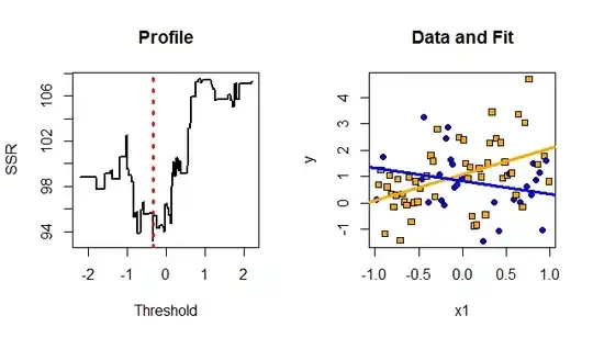
Orange squares and blue circles distinguish the cases $x_2 \lt \tau$ and $x_2 \ge \tau$, respectively. The two subsets of data are separately fit with straight lines.
A full maximum likelihood solution can be obtained by replacing the sum of squared residuals by the negative log likelihood and applying standard MLE methods to obtain confidence regions for the parameters and to test hypotheses about them.
#
# Create a dataset with a specified model.
#
n <- 80
beta <- c(1,1,0,-2)
threshold <- -1/3
sigma <- 1
x1 <- seq(1-n,n-1,2)/n
set.seed(17)
x2 <- rnorm(n)
i <- x2 < threshold
x <- cbind(1, x1, i, x1*i)
y <- x %*% beta + rnorm(n, sd=sigma)
#
# Display the SSR profile for the threshold.
#
f <- function(threshold) lm(y ~ x1*I(x2 < threshold))
z <- seq(-1,1,0.5/n)*2*sd(x2)                   # Search range
w <- sapply(z, function(z) sum(resid(f(z))^2))  # Sum of squares of residuals

par(mfrow=c(1,2))
plot(z, w, lwd=2, type="l", xlab="Threshold", ylab="SSR",main="Profile")
t.opt <- (z[which.min(w)] + z[length(z)+1 - which.min(rev(w))])/2
abline(v=t.opt, lty=3, lwd=3, col="Red")
#
# Fit the model to the data.
#
fit <- f(t.opt)
#
# Report and display the fit.
#
summary(fit)
plot(x1, y, pch=ifelse(x2 < t.opt, 21, 22), bg=ifelse(x2 < t.opt, "Blue", "Orange"),
     main="Data and Fit")
b <- coef(fit)
abline(b[c(1,2)], col="Orange", lwd=3, lty=1)
abline(b[c(1,2)] + b[c(3,4)], col="Blue", lwd=3, lty=1)