Regression of a combined linear model in R

Question

I am trying to combine two linear models (one linear-quadratic and one linear) into one unified model by means of piecewise regression. The tail of the lhs (linear-quadratic part) should continue to be the asymptote for the rhs (linear part). Here's a link! The piecewise function is,

$$y = ax + bx^2,\ x \lt x_t$$ and

$$y = cx + d,\ x \ge x_t$$

where $a, b, c, d$ and $x_t$ (a breakpoint) are parameters to be determined. This unified model should be compared with the linear-quadratic model for the whole range of $x$ by R.squared.adjusted as a measure of goodness of fit.

> y
[1] 1.00000 0.59000 0.15000 0.07800 0.02000 0.00470 0.00190 1.00000 0.56000 0.13000 0.02500 0.00510 0.00160 0.00091 1.00000 0.61000 0.12000
[18] 0.02600 0.00670 0.00085 0.00040
> x
[1] 0.00  5.53 12.92 16.61 20.30 23.07 24.92  0.00  5.53 12.92 16.61 20.30 23.07 24.92  0.00  5.53 12.92 16.61 20.30 23.07 24.92

I'm after continuity of the first derivative and to find the parameters, including determining the breakpoint. Since i want continuity at $x=x_t$, I have rewritten the piecewise function to

$$y = ax + bx^2,\ x \lt x_t$$ and

$$y = ax_t + bx_t^2 + k(x - x_t),\ x \ge x_t$$

where $k$ is a constant. So my attempt goes as follows (assuming I have derived $x_t$ theoretically):

I = ifelse(x < xt, 0, 1)*(x - xt)
x1 = ifelse(x < xt, x, xt)
mod = lm(y ~  x1 + I(x1^2) + I)

But the tail (asymptote) doesn't seem to be parallel to the linear part in the upper range...

Answer 1

Match the slopes at $x_t$. The slope of the quadratic at any point $x$ is $a+2bx$ while the slope of the linear function is constantly $c$. Therefore

$$c = a + 2 b x_t.\tag{1}$$

For the curve to be continuous, the values must also match at $x_t$. Thus

$$c x_t + d = a x_t + b x_t^2.\tag{2}$$

Plugging $(1)$ in for $c$ yields

$$(a + 2 b x_t) x_t + d = a x_t + b x_t^2.$$

The unique solution is

$$d = -bx_t^2.\tag{3}$$

Therefore your curves can be parameterized by $(a,b)$ alone: $c$ and $d$ are completely determined by them and $x_t$. It is convenient to write any such curve as a basic curve plus a correction that is made once $x$ exceeds $x_t$. The correction at any such $x$ must equal $cx+d - (ax + bx^2)$. Plugging in the solutions $(1)$ and $(3)$ gives

$$(a + 2bx_t)x -bx_t^2 - (a x + b x^2) = -b(x- x_t)^2.$$

$y$ may be expressed in terms of an indicator function $\mathcal{I}$ as

$$y(x) = ax + b(x^2 - \mathcal{I}(x \gt x_t)(x-x_t)^2).$$

The parameterization is linear in $(a,b)$. Assuming the errors in $y$ are additive, independent, have zero means, and are homoscedastic, Ordinary Least Squares will work well. The model is nonlinear in $x_t$. If $x_t$ also must be estimated from the data, OLS can be exploited to fit $(a,b)$ for any possible value of $x_t$, thereby reducing the general problem to a one-parameter nonlinear least squares fit. Only solutions with $x_t$ within the range of the $x$ values of the data need be considered. See https://stats.stackexchange.com/a/146976/919 for an example.

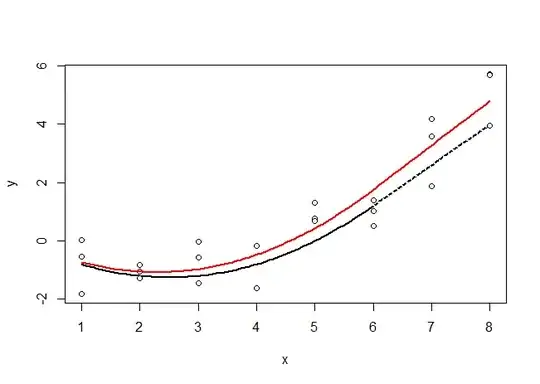
Here is an example showing the true underlying model (in black, with the linear arm dashed), the data, and the fitted model (in red).

The following R code shows how an OLS fit can be computed.

n <- 8      # `x` will range from 1 through `n`
n.rep <- 3  # `y` will be replicated this many times for each `x`
x.t <- 6    # The curves become linear at this value of `x`
a <- -1     # The `x` coefficient
b <- 2/10   # The semi-quadratic coefficient
#
# Synthesize a dataset.
#
set.seed(17)
x <- rep(1:n, n.rep)
y <- a*x + b*f(x, x.t) + rnorm(n*n.rep, sd=1)
#
# Define the family of curves.
# `f` is the "semi-quadratic" function.
#
f <- function(x, x.t) x^2 - (x > x.t)*(x - x.t)^2
#
# Plot the true model and the data.
#
plot(range(x), range(y), type="n", xlab="x", ylab="y")
curve(a*x + b*f(x, x.t), add=TRUE, lwd=2)
curve(a*x + b*f(x, x.t), from=x.t, to=n, add=TRUE, lwd=2, lty=3, col="#e0e0e0")

points(x, y, pch=21, col="Black", bg="#f0f0f0")
#
# Perform an OLS fit and plot it in red.
#
fit <- lm(y ~ -1 + x + I(f(x, x.t)))
a.hat <- coef(fit)[1]
b.hat <- coef(fit)[2]
curve(a.hat*x + b.hat*f(x, x.t), add=TRUE, lwd=2, col="Red")