9

Given a data scatterplot I can plot the data's principal components on it, as axes tiled with points which are principal components scores. You can see an example plot with the cloud (consisting of 2 clusters) and its first principle component. It is drawn easily: raw component scores are computed as data-matrix x eigenvector(s); coordinate of each score point on the original axis (V1 or V2) is score x cos-between-the-axis-and-the-component (which is the element of the eigenvector).

1st principal component tiled by its scores

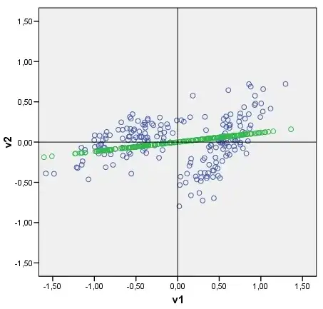
My question: Is it possible somehow to draw a discriminant in a similar fashion? Look at my pic please. I'd like to plot now the discriminant between two clusters, as a line tiled with discriminant scores (after discriminant analysis) as points. If yes, what could be the algo?

ttnphns
  • 51,648
  • 40
  • 253
  • 462

1 Answers1

8

OK, since nobody answered I think that, after some experimentation, I can do it myself. Following discriminant analysis guidelines, let T be the whole cloud's (data X, of 2 variables) sscp matrix (of deviations from cloud's centre), and let W be the pooled within-cluster sscp matrix (of deviations from a cluster centre). B=T-W is the between-cluster sscp matrix. Singular value decomposition of inv(W)B yields us U (left eigenvectors), S (diagonal matrix of eigenvalues), V (right eigenvectors). In my example of 2 clusters only the 1st eigenvalue is nonzero (which means that there is only one discriminant), and so we use only the 1st eigenvector (column) of U: U(1). Now, XU(1) are the sought-for raw discriminant scores. To show the discriminant as a line tiled with those, multiply the scores by cos-between-the-axis-and-the-discriminant (which is the element of the eigenvector U(1)) - just as did it with principal component above. The resulting plot is below.

enter image description here

ttnphns
  • 51,648
  • 40
  • 253
  • 462
  • 1
    It might be easier to think of this as a *projection*: $U(1)$ in both cases (PCA or LDA) is a unit vector in the direction on which you want to project your data (first principle axis, or first "discriminant axis"). Orthogonal projector is [given](http://en.wikipedia.org/wiki/Projection_%28linear_algebra%29#Orthogonal_projections) by $P_U = UU^\top$. So the answer is $XUU^\top$ (which of course is exactly what you found out yourself). The same formula works for higher dimensions as well. – amoeba Jan 25 '14 at 13:45
  • @amoeba, thank you for the comment. The general (for any dimensionality) formula is XV where V is the column-normalized (to SS=1) matrix of eigenvectors of the LDA extraction. These normalized eigenvectors of iris data I display here: http://stats.stackexchange.com/a/83114/3277; the algebra of LDA is here: http://stats.stackexchange.com/a/48859/3277. A plot where I used LDA's normalized eigenvectors is here: http://stats.stackexchange.com/a/22889/3277. – ttnphns Jan 25 '14 at 22:47
  • Yes, sure $XV$ are coordinates of the data points in the target space of lower dimensionality, but if you want to get the image of the projection in the original high-dimensional space (i.e. green dots on your scatter plots in this thread), you project these points back with $V^+$, so in the end you get $XVV^+$. I made a mistake in my previous comment: it reduces to $XVV^\top$ only when $V$ has orthonormal columns, like in the PCA case (but not LDA). Of course if you only consider 1 axis (and so $V$ has only 1 column), then it does not matter. – amoeba Jan 26 '14 at 00:23