8

So let's say I have a bunch of data points in R^n, where n is pretty big (like, 50). I know this data falls into 3 clusters, and I know which cluster each data point is a part of. All I want to do is visualize these clusters in 2D in such a way as to maximize the visual between-clusters separation that I see, with the goal being to prove that the clusters are easily separable based on the location of the data point in R^n alone.

The way I've been going about this up until now involves doing a PCA transform on the data points and then visualizing pairs of PCs at random until I find one where the clusters appear to be pretty cleanly separated. This approach seems pretty ad hoc though, and it seems like there should be an easy way to find a PCA-style rotation of the data that, instead of maximizing overall variance, maximizes inter-cluster separation.

Is there a standard technique out there that does this? If not, any ideas about how to create such a transformation?
dmonner
  • 133
  • 4
  • You might be interested in [Projection Pursuit](http://en.wikipedia.org/wiki/Projection_pursuit). (Available in the [GGobi](http://www.ggobi.org/) software.) – chl Oct 03 '11 at 20:18

5 Answers5

8

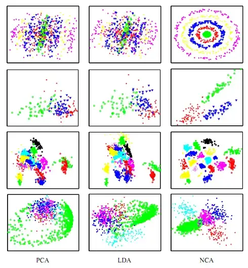
There is two methods that come to my mind which you might be interested in. The first is making use of known clusters and is called 'Neighbourhood components analysis' by Goldberger et al .

The idea is that you learn a mapping (eg affine) from the higher dimensional space to a visualizable space. (eg $A: \mathbb{R}^n \mapsto \mathbb{R}^2$). This mapping is estimated by maximimizing the average number of correct classification if a variation of k-nearest neighbour classification is used. There are some impressive results obtained:

NCA on the wine, faces and digits dataset

The other one is tSNE, which learns a mapping (eg $A: \mathbb{R}^n \mapsto \mathbb{R}^2$). This mapping does not have any constraints, but the loss optimized (not wrt to some parametrization, but with new points in $\mathbb{R}^2$ itself) is that the new space reflects similar distances to the original space. Similar is rather complicated here, it is based on assuming certain distributions of the points in the space and the corresponding KL-divergence.

For the latter, there is matlab code which you can find at the given link. Here is a visualization of the MNIST dataset:

tSNE on MNIST

Andy W
  • 15,245
  • 8
  • 69
  • 191
bayerj
  • 12,735
  • 3
  • 35
  • 56
6

"a PCA-style rotation of the data that, instead of maximizing overall variance, maximizes inter-cluster separation". Discriminant analysis is exactly such a technique. A principal component maximizes variance along it. A discriminant function maximizes ratio between-cluster-variance/pooled-within-cluster-variance along it.

ttnphns
  • 51,648
  • 40
  • 253
  • 462
  • Discriminant analysis is not canonically presented as something that yields a 2d embedding of the data. What 2d embedding do you suggest extracting from, say, Fisher's LDA? – eric_kernfeld Oct 18 '16 at 14:02
  • @eric_kernfeld, one easily plots the data in the space of the discriminant functions. Also, it is easy to show the functions as additional axes within the space of the original variables, such as shown [here](http://stats.stackexchange.com/a/22889/3277) and [here](http://stats.stackexchange.com/q/12861/3277). – ttnphns Oct 18 '16 at 14:11
3

You might want to look at this paper:

G. Sanguinetti, Dimensionality reduction of clustered data sets, IEEE Trans. Pattern Analysis and Machine Intelligence (PAMI) 30(3), 535-540 (2008) (www)

Which describes an unsupervised version of linear discriminant analysis, I have seen some demonstrations of this and it looks like a very useful tool to have in ones toolbox.

If you already know which classes each sample belongs to, then (as ttnphns suggests) you want Linear Discriminant Analysis, Andrew Webb's book on statistical pattern recognition is a good reference book for that kind of thing.

Dikran Marsupial
  • 46,962
  • 5
  • 121
  • 178
0

The article "A Unified Approach to PCA, PLS, MLR and CCA" (by M Borga et al) provides a compact description about various kind of linear projection methods including PCA and LDA.

0

Partial Least Squares will do what you want. The "pls" library in R is what I've traditionally used. Here's an example that creates 3 groups of 50 points, assembles them into a data frame with group labels, and runs PLS on them:

library(MASS)
library(pls)

pts1 = mvrnorm(50,c(3,0,3),diag(c(1,1,1)))
pts2 = mvrnorm(50,c(-3,0,3),diag(c(1,1,1)))
pts3 = mvrnorm(50,c(3,3,-3),diag(c(1,1,1)))
pts = as.data.frame(rbind(pts1,pts2,pts3))

pts$labels = c(rep(1,50),rep(2,50),rep(3,50))

plsresult = plsr(labels~.,ncomp=2,data=pts)
plot(plsresult$scores,col=pts$labels)
chl
  • 50,972
  • 18
  • 205
  • 364