Reproduce linear discriminant analysis projection plot

Question

I'm struggling with projection points in linear discriminant analysis (LDA). Many books on multivariate statistical methods illustrate the idea of the LDA with the figure below.

The problem description is as follows. First we need to draw decision boundary, add perpendicular line and than plot projections of data points on it. I wonder how to add projection points to the perpendicular line.

Any suggestions / pointers?

Answer 1

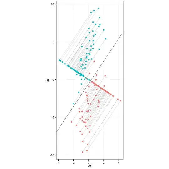
The discriminant axis (the onto which the points are projected on your Figure 1) is given by the first eigenvector of $\mathbf{W}^{-1}\mathbf{B}$. In case of only two classes this eigenvector is proportional to $\mathbf{W}^{-1}(\mathbf{m}_1-\mathbf{m}_2)$, where $\mathbf{m}_i$ are class centroids. Normalize this vector (or the obtained eigenvector) to get the unit axis vector $\mathbf{v}$. This is enough to draw the axis.

To project the (centred) points onto this axis, you simply compute $\mathbf{X}\mathbf{v}\mathbf{v}^\top$. Here $\mathbf{v}\mathbf{v}^\top$ is a linear projector onto $\mathbf{v}$.

Here is the data sample from your dropbox and the LDA projection:

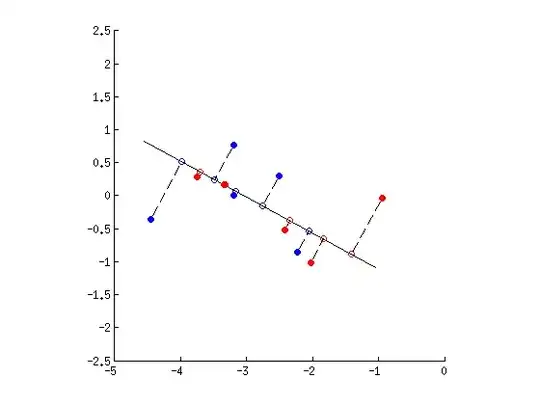
Here is MATLAB code to produce this figure (as requested):

% # data taken from your example
X = [-0.9437    -0.0433; -2.4165    -0.5211; -2.0249    -1.0120; ...
    -3.7482 0.2826; -3.3314 0.1653; -3.1927 0.0043; -2.2233 -0.8607; ...
    -3.1965 0.7736; -2.5039 0.2960; -4.4509 -0.3555];
G = [1 1 1 1 1 2 2 2 2 2];

% # overall mean
mu = mean(X);

% # loop over groups
for g=1:max(G)
    mus(g,:) = mean(X(G==g,:)); % # class means
    Ng(g) = length(find(G==g)); % # number of points per group
end

Sw = zeros(size(X,2)); % # within-class scatter matrix
Sb = zeros(size(X,2)); % # between-class scatter matrix
for g=1:max(G)
    Xg = bsxfun(@minus, X(G==g,:), mus(g,:)); % # centred group data
    Sw = Sw + transpose(Xg)*Xg;
    Sb = Sb + Ng(g)*(transpose(mus(g,:) - mu)*(mus(g,:) - mu));
end

St = transpose(bsxfun(@minus,X,mu)) * bsxfun(@minus,X,mu); % # total scatter matrix
assert(sum(sum((St-Sw-Sb).^2)) < 1e-10, 'Error: Sw + Sb ~= St')

% # LDA
[U,S] = eig(Sw\Sb);

% # projecting data points onto the first discriminant axis
Xcentred = bsxfun(@minus, X, mu);
Xprojected = Xcentred * U(:,1)*transpose(U(:,1));
Xprojected = bsxfun(@plus, Xprojected, mu);

% # preparing the figure
colors = [1 0 0; 0 0 1];
figure
hold on
axis([-5 0 -2.5 2.5])
axis square

% # plot discriminant axis
plot(mu(1) + U(1,1)*[-2 2], mu(2) + U(2,1)*[-2 2], 'k')
% # plot projection lines for each data point
for i=1:size(X,1)
    plot([X(i,1) Xprojected(i,1)], [X(i,2) Xprojected(i,2)], 'k--')
end
% # plot projected points
scatter(Xprojected(:,1), Xprojected(:,2), [], colors(G, :))
% # plot original points
scatter(X(:,1), X(:,2), [], colors(G, :), 'filled')

Answer 2

And "my" solution. Many thanks to @ttnphns and @amoeba!

set.seed(2014)
library(MASS)
library(DiscriMiner) # For scatter matrices
library(ggplot2)
library(grid)
# Generate multivariate data
mu1 <- c(2, -3)
mu2 <- c(2, 5)
rho <- 0.6
s1 <- 1
s2 <- 3
Sigma <- matrix(c(s1^2, rho * s1 * s2, rho * s1 * s2, s2^2), byrow = TRUE, nrow = 2)
n <- 50
# Multivariate normal sampling
X1 <- mvrnorm(n, mu = mu1, Sigma = Sigma)
X2 <- mvrnorm(n, mu = mu2, Sigma = Sigma)
X <- rbind(X1, X2)
# Center data
Z <- scale(X, scale = FALSE)
# Class variable
y <- rep(c(0, 1), each = n)

# Scatter matrices
B <- betweenCov(variables = X, group = y)
W <- withinCov(variables = X, group = y)

# Eigenvectors
ev <- eigen(solve(W) %*% B)$vectors
slope <- - ev[1,1] / ev[2,1]
intercept <- ev[2,1]

# Create projections on 1st discriminant
P <- Z %*% ev[,1] %*% t(ev[,1])

# ggplo2 requires data frame
my.df <- data.frame(Z1 = Z[, 1], Z2 = Z[, 2], P1 = P[, 1], P2 = P[, 2])

plt <- ggplot(data = my.df, aes(Z1, Z2))
plt <- plt + geom_segment(aes(xend = P1, yend = P2), size = 0.2, color = "gray")
plt <- plt + geom_point(aes(color = factor(y)))
plt <- plt + geom_point(aes(x = P1, y = P2, colour = factor(y)))
plt <- plt + scale_colour_brewer(palette = "Set1")
plt <- plt + geom_abline(intercept = intercept, slope = slope, size = 0.2)
plt <- plt + coord_fixed()
plt <- plt + xlab(expression(X[1])) + ylab(expression(X[2]))
plt <- plt + theme_bw()
plt <- plt + theme(axis.title.x = element_text(size = 8),
                   axis.text.x  = element_text(size = 8),
                   axis.title.y = element_text(size = 8),
                   axis.text.y  = element_text(size = 8),
                   legend.position = "none")
plt