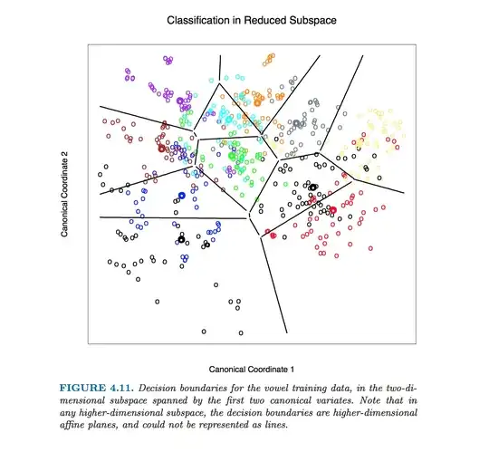
This particular figure in Hastie et al. was produced without computing equations of class boundaries. Instead, algorithm outlined by @ttnphns in the comments was used, see footnote 2 in section 4.3, page 110:
For this figure and many similar figures in the book we compute the decision boundaries by an exhaustive contouring method. We compute the decision rule on a fine lattice of points, and then use contouring algorithms to compute the boundaries.
However, I will proceed with describing how to obtain equations of LDA class boundaries.
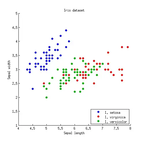
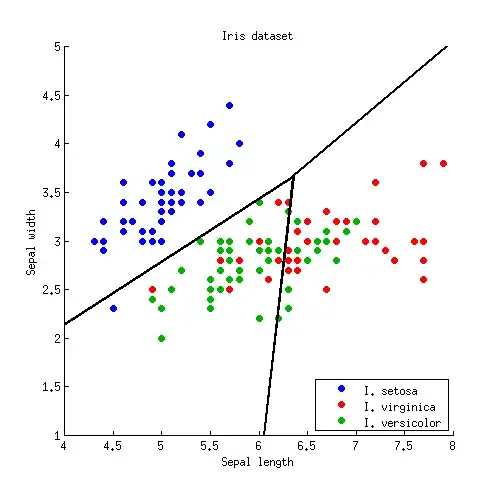
Let us start with a simple 2D example. Here is the data from the Iris dataset; I discard petal measurements and only consider sepal length and sepal width. Three classes are marked with red, green and blue colours:
Let us denote class means (centroids) as $\boldsymbol\mu_1, \boldsymbol\mu_2, \boldsymbol\mu_3$. LDA assumes that all classes have the same within-class covariance; given the data, this shared covariance matrix is estimated (up to the scaling) as $\mathbf{W} = \sum_i (\mathbf{x}_i-\boldsymbol \mu_k)(\mathbf{x}_i-\boldsymbol \mu_k)^\top$, where the sum is over all data points and centroid of the respective class is subtracted from each point.
For each pair of classes (e.g. class $1$ and $2$) there is a class boundary between them. It is obvious that the boundary has to pass through the middle-point between the two class centroids $(\boldsymbol \mu_{1} + \boldsymbol \mu_{2})/2$. One of the central LDA results is that this boundary is a straight line orthogonal to $\mathbf{W}^{-1} \boldsymbol (\boldsymbol \mu_{1} - \boldsymbol \mu_{2})$. There are several ways to obtain this result, and even though it was not part of the question, I will briefly hint at three of them in the Appendix below.
Note that what is written above is already a precise specification of the boundary. If one wants to have a line equation in the standard form $y=ax+b$, then coefficients $a$ and $b$ can be computed and will be given by some messy formulas. I can hardly imagine a situation when this would be needed.
Let us now apply this formula to the Iris example. For each pair of classes I find a middle point and plot a line perpendicular to $\mathbf{W}^{-1}
\boldsymbol (\boldsymbol \mu_{i} - \boldsymbol \mu_{j})$:
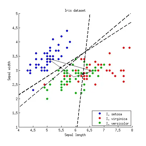
Three lines intersect in one point, as should have been expected. Decision boundaries are given by rays starting from the intersection point:
Note that if the number of classes is $K\gg 2$, then there will be $K(K-1)/2$ pairs of classes and so a lot of lines, all intersecting in a tangled mess. To draw a nice picture like the one from the Hastie et al., one needs to keep only the necessary segments, and it is a separate algorithmic problem in itself (not related to LDA in any way, because one does not need it to do the classification; to classify a point, either check the Mahalanobis distance to each class and choose the one with the lowest distance, or use a series or pairwise LDAs).
In $D>2$ dimensions the formula stays exactly the same: boundary is orthogonal to $\mathbf{W}^{-1} \boldsymbol (\boldsymbol \mu_{1} - \boldsymbol \mu_{2})$ and passes through $(\boldsymbol \mu_{1} + \boldsymbol \mu_{2})/2$. However, in higher dimensions this is not a line anymore, but a hyperplane of $D-1$ dimensions. For illustration purposes, one can simply project the dataset to the first two discriminant axes, and thus reduce the problem to the 2D case (that I believe is what Hastie et al. did to produce that figure).
Appendix
How to see that the boundary is a straight line orthogonal to $\mathbf{W}^{-1} (\boldsymbol \mu_{1} - \boldsymbol \mu_{2})$? Here are several possible ways to obtain this result:
The fancy way: $\mathbf{W}^{-1}$ induces Mahalanobis metric on the plane; the boundary has to be orthogonal to $\boldsymbol \mu_{1} - \boldsymbol \mu_{2}$ in this metric, QED.
The standard Gaussian way: if both classes are described by Gaussian distributions, then the log-likelihood that a point $\mathbf x$ belongs to class $k$ is proportional to $(\mathbf x - \boldsymbol \mu_k)^\top \mathbf W^{-1}(\mathbf x - \boldsymbol \mu_k)$. On the boundary the likelihoods of belonging to classes $1$ and $2$ are equal; write it down, simplify, and you will immediately get to $\mathbf x^\top \mathbf W^{-1} (\boldsymbol \mu_{1} - \boldsymbol \mu_{2}) = \mathrm{const}$, QED.
The laboursome but intuitive way. Imagine that $\mathbf{W}$ is an identity matrix, i.e. all classes are spherical. Then the solution is obvious: boundary is simply orthogonal to $\boldsymbol \mu_1 - \boldsymbol \mu_2$. If classes are not spherical, then one can make them such by sphering. If the eigen-decomposition of $\mathbf{W}$ is $\mathbf{W} = \mathbf U \mathbf D \mathbf U^\top$, then matrix $\mathbf S = \mathbf D^{-1/2} \mathbf U^\top$ will do the trick (see e.g. here). So after applying $\mathbf S$, the boundary is orthogonal to $\mathbf S (\boldsymbol \mu_{1} - \boldsymbol \mu_{2})$. If we take this boundary, transform it back with $\mathbf S^{-1}$ and ask what is it now orthogonal to, the answer (left as an exercise) is: to $\mathbf S^\top \mathbf S \boldsymbol (\boldsymbol \mu_{1} - \boldsymbol \mu_{2})$. Plugging in the expression for $\mathbf S$, we get QED.