13

I have dataset with assumption that nearest neighbors are best predictors. Just a perfect example of two-way gradient visualized-

enter image description here

Suppose we have case where few values are missing, we can easily predict based on neighbors and trend.

enter image description here

Corresponding data matrix in R (dummy example for workout):

miss.mat <- matrix (c(5:11, 6:10, NA,12, 7:13, 8:14, 9:12, NA, 14:15, 10:16),ncol=7, byrow = TRUE)
miss.mat 
    [,1] [,2] [,3] [,4] [,5] [,6] [,7]
[1,]    5    6    7    8    9   10   11
[2,]    6    7    8    9   10   NA   12
[3,]    7    8    9   10   11   12   13
[4,]    8    9   10   11   12   13   14
[5,]    9   10   11   12   NA   14   15
[6,]   10   11   12   13   14   15   16

Notes: (1) The property of missing values is assumed to be random, it can happen anywhere.

(2) All data points are from single variable, but their value are assumed to be influenced by neighbors in row and column adjacent to them. So position in matrix is important and may be considered as other variable.

My hope in some situations I can predict some off-values (may be mistakes) and correct bias (just example, lets generate such error in the dummy data) :

> mat2 <- matrix (c(4:10, 5, 16, 7, 11, 9:11, 6:12, 7:13, 8:14, 9:13, 4,15, 10:11, 2, 13:16),ncol=7, byrow = TRUE)
> mat2

    [,1] [,2] [,3] [,4] [,5] [,6] [,7]
[1,]    4    5    6    7    8    9   10
[2,]    5   16    7   11    9   10   11
[3,]    6    7    8    9   10   11   12
[4,]    7    8    9   10   11   12   13
[5,]    8    9   10   11   12   13   14
[6,]    9   10   11   12   13    4   15
[7,]   10   11    2   13   14   15   16

The above examples are just illustration (may be answered visually) but the real example may be more confusing. I am looking if there is robust method to do such analysis. I think this should be possible. What would be suitable method to perform this type of analysis ? any R program / package suggestions to do this type of analysis ?

enter image description here

rdorlearn
  • 3,493
  • 6
  • 26
  • 29

2 Answers2

7

The question asks for ways to use nearest neighbors in a robust way to identify and correct localized outliers. Why not do exactly that?

The procedure is to compute a robust local smooth, evaluate the residuals, and zero out any that are too large. This satisfies all the requirements directly and is flexible enough to adjust to different applications, because one can vary the size of the local neighborhood and the threshold for identifying outliers.

(Why is flexibility so important? Because any such procedure stands a good chance of identifying certain localized behaviors as being "outlying". As such, all such procedures can be considered smoothers. They will eliminate some detail along with the apparent outliers. The analyst needs some control over the trade-off between retaining detail and failing to detect local outliers.)

Another advantage of this procedure is that it does not require a rectangular matrix of values. In fact, it can even be applied to irregular data by using a local smoother suitable for such data.

R, as well as most full-featured statistics packages, has several robust local smoothers built in, such as loess. The following example was processed using it. The matrix has $79$ rows and $49$ columns--almost $4000$ entries. It represents a complicated function having several local extrema as well as an entire line of points where it is not differentiable (a "crease"). To slightly more than $5\%$ of the points--a very high proportion to be considered "outlying"--were added Gaussian errors whose standard deviation is only $1/20$ of the standard deviation of the original data. This synthetic dataset thereby presents many of the challenging features of realistic data.

Figures

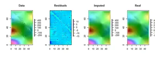
Note that (as per R conventions) the matrix rows are drawn as vertical strips. All images, except for the residuals, are hillshaded to help display small variations in their values. Without this, almost all the local outliers would be invisible!

By comparing the "Imputed" (fixed up) to the "Real" (original uncontaminated) images, it is evident that removing the outliers has smoothed out some, but not all, of the crease (which runs from $(0,79)$ down to $(49, 30)$; it is apparent as a light cyan angled stripe in the "Residuals" plot).

The speckles in the "Residuals" plot show the obvious isolated local outliers. This plot also displays other structure (such as that diagonal stripe) attributable to the underlying data. One could improve on this procedure by using a spatial model of the data (via geostatistical methods), but describing that and illustrating it would take us too far afield here.

BTW, this code reported finding only $102$ of the $200$ outliers that were introduced. This is not a failure of the procedure. Because the outliers were Normally distributed, about half of them were so close to zero--$3$ or less in size, compared to underlying values having a range of over $600$--that they made no detectable change in the surface.

#
# Create data.
#
set.seed(17)
rows <- 2:80; cols <- 2:50
y <- outer(rows, cols, 
           function(x,y) 100 * exp((abs(x-y)/50)^(0.9)) * sin(x/10) * cos(y/20))
y.real <- y
#
# Contaminate with iid noise.
#
n.out <- 200
cat(round(100 * n.out / (length(rows)*length(cols)), 2), "% errors\n", sep="")
i.out <- sample.int(length(rows)*length(cols), n.out)
y[i.out] <- y[i.out] + rnorm(n.out, sd=0.05 * sd(y))
#
# Process the data into a data frame for loess.
#
d <- expand.grid(i=1:length(rows), j=1:length(cols))
d$y <- as.vector(y)
#
# Compute the robust local smooth.
# (Adjusting `span` changes the neighborhood size.)
#
fit <- with(d, loess(y ~ i + j, span=min(1/2, 125/(length(rows)*length(cols)))))
#
# Display what happened.
#
require(raster)
show <- function(y, nrows, ncols, hillshade=TRUE, ...) {
  x <- raster(y, xmn=0, xmx=ncols, ymn=0, ymx=nrows)
  crs(x) <- "+proj=lcc +ellps=WGS84"
  if (hillshade) {
    slope <- terrain(x, opt='slope')
    aspect <- terrain(x, opt='aspect')
    hill <- hillShade(slope, aspect, 10, 60)
    plot(hill, col=grey(0:100/100), legend=FALSE, ...)
    alpha <- 0.5; add <- TRUE
  } else {
    alpha <- 1; add <- FALSE
  }
  plot(x, col=rainbow(127, alpha=alpha), add=add, ...)
}

par(mfrow=c(1,4))
show(y, length(rows), length(cols), main="Data")

y.res <- matrix(residuals(fit), nrow=length(rows))
show(y.res, length(rows), length(cols), hillshade=FALSE, main="Residuals")
#hist(y.res, main="Histogram of Residuals", ylab="", xlab="Value")

# Increase the `8` to find fewer local outliers; decrease it to find more.
sigma <- 8 * diff(quantile(y.res, c(1/4, 3/4)))
mu <- median(y.res)
outlier <- abs(y.res - mu) > sigma
cat(sum(outlier), "outliers found.\n")

# Fix up the data (impute the values at the outlying locations).
y.imp <- matrix(predict(fit), nrow=length(rows))
y.imp[outlier] <- y[outlier] - y.res[outlier]

show(y.imp, length(rows), length(cols), main="Imputed")
show(y.real, length(rows), length(cols), main="Real")
whuber
  • 281,159
  • 54
  • 637
  • 1,101
  • whuber: Do I understand it correctly that you assume that the outliers are isolated cells? If so, would you know how sensitive is this approach to violation of this assumption? – user603 May 28 '14 at 21:30
  • @user603 I do not assume the outliers are isolated--many of them in the example are not--but I do assume that the proportion of outliers in any local neighborhood is low enough that they will not break down the local smoother. Arguably, if there is any neighborhood with a very large proportion of such outliers, they can no longer be considered local outliers! – whuber May 28 '14 at 21:37
  • Thanks for the clarification. I just realized that in the procedure I describe, the data needs to be standardized first so that each column has the same (robust) scale. I wonder whether the procedure you describe should not also include one such step (I apologize and will remove my comment if I missed this detail in your exposition). – user603 May 28 '14 at 21:39
  • @user603 In the general setting, where there are missing values or the data are irregularly spaced, a preliminary standardization cannot be applied. Where it can be, but nothing else is assumed of the data, I see little harm ni it--provided the location and scale are estimated with robust methods. In fact, in such cases analysts might begin with a *median polish* of the matrix and only then start examining its residuals for further structure and outliers. John Tukey illustrates this (in a limited fashion) in *EDA* and Noel Cressie advocated it for spatial data analysis about 25 years ago. – whuber May 28 '14 at 21:45
  • (Cont'd) If there is no expectation of stationary-like behavior in the dataset, though, then nothing seems to be gained by a preliminary standardization of rows or columns. Therefore I (purposely) omitted any mention of such a process. – whuber May 28 '14 at 21:46
  • but then, if some columns are measured in vastly different scales than adjacent ones, doesn't that compromise the 'local' smoothing approach? Or is the local smoothing only performed on each column independently? – user603 May 28 '14 at 21:51
  • 1
    @user603 Absolutely! But that seems to take us out of the presumptive situation where "nearest neighbors are best predictors." Out of respect for that, anything we do when processing the data should preserve this local predictability. If one column has a "vastly different scale" than its neighbor, that circumstance would violate this stated assumption pretty strongly. (I also wonder at your focus on columns: upon re-reading the question, I cannot detect any asymmetry in the roles of columns and rows.) – whuber May 28 '14 at 21:55
  • 1
    @user603 I think I now see where you're coming from: one can understand the question as dealing with a matrix of *cases* (=rows) and *attributes* (or "fields" or "factors" or "variables", all in columns); that the cases can be conceived of as representing (irregularly spaced) points in a $p$-dimensional space; and that "nearest neighbors" are understood in terms of a natural metric on this space. That's a completely different interpretation than mine and the two interpretations cannot easily be related, because your missing values or outliers affect the very *locations* of these points. – whuber May 28 '14 at 22:01
  • I agree. For example, as I understand it, the alternating PCA rotations in the approach I describe are used to mitigate the effect of the initial colum-wise scaling on the final fit. Of course If you take the notion of neighbourhood literally (as in the interpretation you make) the original scaling and the ensuing PCA's are not so crucial. On a different note, PCA is also performing a shrinkage (but again in a metric that is not based on a similar definition of neighbourhood as for the loess fits). – user603 May 28 '14 at 22:07
  • In my situation is matrix of rows and columns, both rows and columns can have effect - the effect may be local and/or global - in any situation the neighbors in rows or column direction are best predictors of missing value or plays role in identification of mistakes. – rdorlearn May 29 '14 at 02:26
  • 1
    @whuber this is great solution, thanks - I was trying to introduce at least some missing values, which is always real situation - a mix of missing (for example 50 missing value) and outliers (100 outliers). exciting ! – rdorlearn May 29 '14 at 03:02
4

I would advise you to have a look at this article [0]. The problem it purports to address seems to fit your description of yours rather well, except that the method proposed by the author is slightly more refined than NN-inputation (although it uses something similar as a starting point).

(throughout, I will assume that $\pmb X$, the $n$ by $p$ data matrix has been standardized: each column has been divide by the mad in the pre-processing step of the analysis)

The idea of this approach is to obtain a rank $k$ robust PCA decomposition of your data matrix in a way that is resistant to the possible presence of outliers (this is done by using a bounded loss function when estimating the PCA components) and missing values (this is done by using an EM-type imputation method). As I explain below, once you have such a PCA decomposition of your dataset, filling in the missing elements (and assessing the uncertainty around these estimates is pretty straightforward).

The first step of each iteration is the data imputation step. This is done as in the EM algorithm: the missing cells are filled by the value which they are expected to have (this is the E-step).

In the second part of the two step iterative procedure, one fits a (robust) PCA to the augmented data obtained from the previous step. This results in a spectral decomposition of $\pmb X$ into $\pmb t\in\mathbb{R}^p$ (an estimate of center), a $p$ by $k$ orthogonal matrix $\pmb L$ and a $k$ by $k$ diagonal matrix $\pmb D$ (with $k\leq p$), which is a sort of robustified, PCA based, M-step.

To summarize the paper, here is the general algorithm they propose:

  • Set $l=0$. Obtain an estimate $\pmb W^0$ where the missing elements are filled with the initial estimates. For each missing cell, these initial estimates are the averages of the row-wise and the column-wise medians of the non missing elements of $\pmb X$ (the original data matrix).

  • Then, do until convergence:

    a. do robust PCA on $\pmb W^l$ and obtain the estimates $(\pmb t^l,\pmb L^l,\pmb D^l)$

    b. set $l=l+1$

    c. use $\pmb Y^{l}=\pmb L^{l-1}(\pmb W^{l-1}-\pmb t^{l-1}) (\pmb L^{l-1})'$

    d. fill the missing elements of $\pmb W^{l}$ by what they are expected to be based on the model $\pmb W^{l}\sim\mathcal{N}(\pmb t^{l-1},\pmb L^{l-1} \pmb D^{l-1}(\pmb L^{l-1})')$ (as in the E step of the EM algorithm) and the non missing elements by the corresponding entries of $\pmb Y^{l}$.

Iterate (a->c) until $||\pmb W^{l-1}-\pmb W^l||_F$ is smaller than some threshold. The vector of estimated parameter obtained at the final iteration are stored as $(\pmb t,\pmb L,\pmb D)$.

The idea, is that at each iteration, the model for the data $(\pmb t^{l-1},\pmb L^{l-1} \pmb D^{l-1})$ moves increasingly further away from the naive, initial estimates while the robust M step prevents the outliers from influencing the fitted parameter.

This approach also gives you a host of diagnostic tool to check the quality of the imputation. For example, you could also produce multiple draws from $\mathcal{N}(\pmb t^{l-1},\pmb L\pmb D(\pmb L)')$ but this time for the non missing elements of your data-matrix and see how much the distribution of the generated (counter-factual) data matches the observed value for each of the non missing cells.

I don't know of a ready made R implementation for this approach, but one can easily be produced from the sub-components (chiefly a robust PCA algorithm), and these are well implemented in R, see the rrcov package (the paper is quiet informative on this subject).

  • [0] Serneels S. and Verdonck, T. (2008). Principal component analysis for data containing outliers and missing elements. Computational Statistics & Data Analysis vol:52 issue:3 pages:1712-1727.
user603
  • 21,225
  • 3
  • 71
  • 135
  • thanks, my objective is here is not to predict outliers (in sense they are away from the distribution) rather off-values (outliers) not fitting to pattern. – rdorlearn May 28 '14 at 12:58
  • I think you misunderstood my answer. This approach will produce prediction for any value, but the outliers will not be predicted very well: this is because they are not permitted to influence the PCA fit. I advise you to read the paper. – user603 May 28 '14 at 12:59
  • thanks, the approach seems interesting and guess may work well too. But without proper codes will be difficult to implement - too sophisticated for me at least ! – rdorlearn May 29 '14 at 03:13