Background subtraction for signal and error analysis

Question

I use a CCD to see the split of a energy level due to Zeeman effect.

I have a 1 dimensional CCD of 7926 pixel of 7μm each one. My CCD analyze a region 2 dimensional, and then it steps forward 200 times. So, i have a matrix like this .

I select the background between 40 and 60 pixel and i calculate for each row the mean value. Then, i project these 7926 mean values over the Y axis. So, for each bins of the row of the matrix(i.e. 3040) , i subtract the value of the content of 3040 pixel of the background

This is my background:

(in x there are the pixels of my CCD and y is the intensity).

I have to subtract the background from the signal, subtracting bin for bin. At each bins of the background it is associated an error $\sigma = \sqrt{N}$ where $N$ is the bin content.

Each bins of the signal has an error $\sqrt{N}$, but when i subtract the backgroun how can i calculate the exact error of the pure signal? If $Z'_i$ is the bin content after the subtraction, $Z_i$ the bin content before and $Y_i$ the bin content of the background, then $Z'_i = Z_i - Y_i$ and the error (throw the propagation) $\sigma_{Y_i} = \sqrt{\sigma_{Z'_i}^2 + \sigma_{Y_i}^2 +....}$

In fact, I think, there should be a term of covariance. How can i compute it?

Answer 1

Estimating that error correctly will be tricky. But I would like to suggest it is more important first to find a better procedure to subtract background. Only once a good procedure is available would it be worthwhile analyzing the amount of error.

In this case, using the mean is biased upwards by the contributions from the signal, which look large enough to be important. Instead use a more robust estimator. A simple one is the median. Moreover, a little more can be squeezed out of these data by adjusting the columns as well as the rows at the same time. This is called "median polish." It is very fast to carry out and is available in some software (such as R).

These figures of simulated data with 793 rows and 200 columns show the result of adjusting background with median polish. (Ignore the labels on the y-axis; they are an artifact of the software used to display the data.)

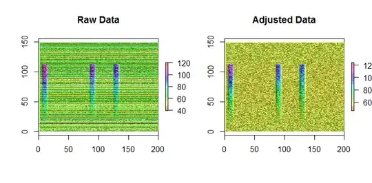
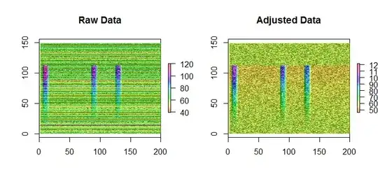
A very slight bias is still evident in the adjusted data: the top and bottom quarters, where the signal is not present in any column, are slightly greener than the middle half. However, by contrast, merely subtracting row means from the data produces obvious bias:

Scatterplots (not shown here, but produced by the code) of actual background against estimated background confirm the superiority of median polish.

Now, this is somewhat an unfair comparison, because to compute background you have previously selected columns believed not to have a signal. But there are problems with this:

• If there are low-level signals present in those areas (which you haven't seen or expected), they will bias the results.

• Only a small subset of the data has been used, magnifying the estimation error in background. (Using only one-tenth of the available columns approximately triples the error in estimating background compared to using the nine-tenths of columns that appear to have little or no signal.)

Furthermore, even when you are confident that some columns do not contain signals, you can still apply median polish to those columns. This will protect you from unexpected violations of your expectations (that these are signal-free areas). Moreover, this robustness will allow you to broaden the set of columns used to estimate background, because if you inadvertently include a few with some signal, they will have only a negligible effect.

Additional processing to identify isolated outliers and to estimate and extract the signal can be done, perhaps in the spirit of my answer to a recent related question.

---

R code:

#
# Create background.
#
set.seed(17)
i <- 1:793
row.sd <- 0.08
row.mean <- log(60) - row.sd^2/2
background <- exp(rnorm(length(i), row.mean, row.sd))
k <- sample.int(length(background), 6)
background[k] <- background[k] * 1.7

par(mfrow=c(1,1))
plot(background, type="l", col="#000080")
#
# Create a signal.
#
j <- 1:200
f <- function(i, j, center, amp=1, hwidth=5, l=0, u=6000) {
  0.2*amp*outer(dbeta((i-l)/(u-l), 3, 1.1), pmax(0, 1-((j-center)/hwidth)^4))
}
#curve(f(x, 10, center=10), 0, 6000)
#image(t(f(i,j, center=100,u=600)), col=c("White", rainbow(100)))

u <- 600
signal <- f(i,j, center=10, amp=110, u=u) +
  f(i,j, center=90, amp=90, u=u) +
  f(i,j, center=130, amp=80, u=u)
#
# Combine signal and background, both with some iid multiplicative error.
#
ccd <- outer(background, j, function(i,j) i) * exp(rnorm(length(signal), sd=0.05)) + 
  signal * exp(rnorm(length(signal), sd=0.1))
ccd <- matrix(pmin(120, ccd), nrow=length(i))
#image(j, i, t(ccd), col=c(rep("#f8f8f8",20), rainbow(100)),main="CCD")
#
# Compute background via row means (not recommended).
# (Returns $row and $overall to match the values of `medpolish`.)
#
mean.subtract <- function(x) {
  row <- apply(x, 1, mean)
  overall <- mean(row)
  row <- row - overall
  return(list(row=row, overall=overall))
}
#
# Estimate background and adjust the image.
#
fit <- medpolish(ccd)
#fit <- mean.subtract(ccd)
ccd.adj <- ccd - outer(fit$row, j, function(i,j) i)
image(j, i, t(ccd.adj), col=c(rep("#f8f8f8",20), rainbow(100)), 
      main="Background Subtracted")
plot(fit$row + fit$overall, type="l", xlab="i")
plot(background, fit$row)
#
# Plot the results.
#
require(raster)
show <- function(y, nrows, ncols, hillshade=TRUE, aspect=1, ...) {
  x <- apply(y, 2, rev)
  x <- raster(x, xmn=0, xmx=ncols, ymn=0, ymx=nrows*aspect)
  crs(x) <- "+proj=lcc +ellps=WGS84"
  if (hillshade) {
    slope <- terrain(x, opt='slope')
    aspect <- terrain(x, opt='aspect')
    hill <- hillShade(slope, aspect, 10, 60)
    plot(hill, col=grey(0:100/100), legend=FALSE, ...)
    alpha <- 0.5; add <- TRUE
  } else {
    alpha <- 1; add <- FALSE
  }
  plot(x, col=rainbow(127, alpha=alpha), add=add, ...)
}

par(mfrow=c(1,2))
asp <- length(j)/length(i) * 6/8
show(ccd, length(i), length(j), aspect=asp, main="Raw Data")
show(ccd.adj, length(i), length(j), aspect=asp, main="Adjusted Data")

Answer 2

On the background computation: Since what you are doing is to measure the background by calculating the average of some values with backgroung only, you can use the error on the average ($\sigma_{Bckg}/\sqrt{n_{avg}}$) and this should estimate correctly the background variation, taking into account the variation of the background among the $n_{avg}$ pixels you considered.

You can also calculate the $Z_i$ error, if I understood correctly, and it is given by $\sqrt{N}$, so this is settled to. In order to calculate the covariance between the errors maybe you can use the covariance formula (and take a look here for an example on the covariance between two variables). I am not the most knowledgeable person about it, so I hope this rambling attract more educated people to the discussion. =)