Assume I have data looking like this
head(dt)

      Mass    RT       A
1 294.9862 6.157 2013154
2 264.0223 6.202  230690
3 283.9639 6.354   65035
4 261.9819 6.362 1607568
5 289.9770 6.480   26762
6 264.0221 6.520  190739

library(ggplot2)
ggplot( data = dt, aes( x = RT, y = Mass ) ) +
  geom_density2d( alpha = 0.8, , h = c(0.1, 1.3) ) +
  geom_point( aes( colour = log2(A)), size = 5  ) +
  scale_color_gradientn( "ld( A )", colours= rev(heat.colors(255)) ) +
  theme_bw()
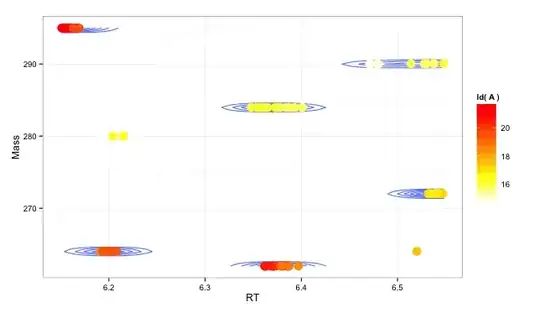
What I want do is to group the points of my data by a kernel density method (as indicated by the density layer of the plot). But I do not really have an idea how to achieve this in R.
I used already npudens from the np package, but did not even really understand how to extract/find the density values from the resulting object.
library(np)
npudens( ~RT+Mass,data=test.tab )
The reason why I choose npudens over kde2d is, that I'd also like to provide conditional bandwidths to the density estimator, i.e. in a way that the bandwidths are linear functions of Mass and RT as for example 0.005% of the mass and 5% of the RT. Any help is highly appreciated. I am new to these methods and feel a little bit lost.
For reproduction here is the dput of my data:
dt <- structure(list(Mass = c(294.9862, 264.0223, 283.9639, 261.9819,
289.977, 264.0221, 272.0176, 294.986, 264.0221, 283.9639, 261.9818,
290.0401, 272.0176, 294.9861, 264.0222, 283.9636, 261.9819, 272.0176,
294.9862, 283.9635, 261.9818, 289.977, 272.0173, 294.9863, 283.964,
261.9818, 290.0397, 272.0174, 294.9861, 283.9641, 261.9819, 289.9764,
290.0398, 272.0174, 294.9862, 264.0222, 283.9637, 261.9818, 289.9769,
290.0402, 272.0174, 294.9861, 264.0223, 279.9958, 283.9637, 261.9818,
289.9766, 290.0401, 272.0174, 294.9862, 264.0222, 283.9638, 261.9819,
290.04, 272.0172, 294.9861, 283.9638, 261.9819, 289.9769, 290.04,
272.0173, 294.9862, 264.0223, 261.9819, 290.0401, 272.0175, 294.9862,
264.0224, 283.9637, 261.982, 272.0173, 294.9862, 283.9635, 261.9816,
290.0402, 272.0172, 294.9861, 264.0222, 279.9961, 283.9637, 261.9815,
272.0171, 294.9862, 264.0222, 283.9638, 261.9818, 272.0174, 294.9859,
264.0224, 283.9638, 272.0169, 294.986, 264.0225, 283.9636, 272.017,
294.9861, 264.0225, 283.9635, 272.0168, 290.0401), RT = c(6.157,
6.202, 6.354, 6.362, 6.48, 6.52, 6.543, 6.153, 6.193, 6.348,
6.362, 6.514, 6.54, 6.153, 6.191, 6.359, 6.368, 6.542, 6.161,
6.362, 6.37, 6.479, 6.546, 6.157, 6.359, 6.371, 6.528, 6.544,
6.151, 6.355, 6.363, 6.471, 6.528, 6.539, 6.159, 6.205, 6.365,
6.372, 6.472, 6.529, 6.54, 6.155, 6.2, 6.204, 6.373, 6.38, 6.479,
6.529, 6.539, 6.161, 6.202, 6.373, 6.386, 6.538, 6.547, 6.163,
6.376, 6.387, 6.472, 6.537, 6.54, 6.156, 6.194, 6.374, 6.529,
6.532, 6.155, 6.193, 6.377, 6.382, 6.532, 6.162, 6.362, 6.379,
6.53, 6.534, 6.165, 6.198, 6.215, 6.387, 6.387, 6.539, 6.166,
6.201, 6.378, 6.397, 6.541, 6.169, 6.208, 6.393, 6.54, 6.163,
6.203, 6.384, 6.542, 6.164, 6.201, 6.401, 6.535, 6.548), A = c(2013154,
230690, 65035, 1607568, 26762, 190739, 121136, 2357853, 263807,
68086, 1551442, 59292, 118160, 2529240, 313389, 64018, 1519476,
119259, 2984633, 80162, 1680411, 35609, 157181, 3182405, 81694,
1721163, 49815, 152731, 3283306, 76425, 1623899, 35616, 45969,
155354, 2859136, 630649, 80974, 1435648, 30731, 50551, 160070,
3190792, 679125, 72635, 83406, 1190889, 32199, 48741, 153469,
3188184, 662134, 81513, 1066302, 54851, 151038, 2883657, 68430,
974675, 28558, 48020, 146510, 3052724, 679433, 1242839, 55651,
137011, 3178104, 702678, 62029, 903551, 149964, 2448393, 62758,
461936, 51645, 138286, 2492192, 736078, 91805, 67877, 450461,
146526, 2678001, 731678, 57059, 355304, 147477, 756005, 686878,
58532, 120400, 841196, 754836, 52527, 115968, 862693, 742445,
53013, 111391, 68416)), .Names = c("Mass", "RT", "A"), row.names = c(NA,
-100L), class = "data.frame")