Interpolation of influenza data that conserves weekly mean

Question

Edit

I have found a paper describing exactly the procedure I need. The only difference is that the paper interpolates monthly mean data to daily, while preserving the monthly means. I have trouble to implement the approach in R. Any hints are appreciated.

Original

For each week, I have the following count data (one value per week):

Number of doctors' consultations
Number of cases of influenza

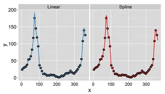
My goal is to obtain daily data by interpolation (I thought of linear or truncated splines). The important thing is that I want to conserve the weekly mean, i.e. the mean of the daily interpolated data should equal the recorded value of this week. In addition, the interpolation should be smooth. One problem that could arise is that a certain week has less than 7 days (e.g. at the beginning or end of a year).

I would be grateful for advice on this matter.

Thanks a lot.

Here's a sample data set for the year 1995 (updated):

structure(list(daily.ts = structure(c(9131, 9132, 9133, 9134, 
9135, 9136, 9137, 9138, 9139, 9140, 9141, 9142, 9143, 9144, 9145, 
9146, 9147, 9148, 9149, 9150, 9151, 9152, 9153, 9154, 9155, 9156, 
9157, 9158, 9159, 9160, 9161, 9162, 9163, 9164, 9165, 9166, 9167, 
9168, 9169, 9170, 9171, 9172, 9173, 9174, 9175, 9176, 9177, 9178, 
9179, 9180, 9181, 9182, 9183, 9184, 9185, 9186, 9187, 9188, 9189, 
9190, 9191, 9192, 9193, 9194, 9195, 9196, 9197, 9198, 9199, 9200, 
9201, 9202, 9203, 9204, 9205, 9206, 9207, 9208, 9209, 9210, 9211, 
9212, 9213, 9214, 9215, 9216, 9217, 9218, 9219, 9220, 9221, 9222, 
9223, 9224, 9225, 9226, 9227, 9228, 9229, 9230, 9231, 9232, 9233, 
9234, 9235, 9236, 9237, 9238, 9239, 9240, 9241, 9242, 9243, 9244, 
9245, 9246, 9247, 9248, 9249, 9250, 9251, 9252, 9253, 9254, 9255, 
9256, 9257, 9258, 9259, 9260, 9261, 9262, 9263, 9264, 9265, 9266, 
9267, 9268, 9269, 9270, 9271, 9272, 9273, 9274, 9275, 9276, 9277, 
9278, 9279, 9280, 9281, 9282, 9283, 9284, 9285, 9286, 9287, 9288, 
9289, 9290, 9291, 9292, 9293, 9294, 9295, 9296, 9297, 9298, 9299, 
9300, 9301, 9302, 9303, 9304, 9305, 9306, 9307, 9308, 9309, 9310, 
9311, 9312, 9313, 9314, 9315, 9316, 9317, 9318, 9319, 9320, 9321, 
9322, 9323, 9324, 9325, 9326, 9327, 9328, 9329, 9330, 9331, 9332, 
9333, 9334, 9335, 9336, 9337, 9338, 9339, 9340, 9341, 9342, 9343, 
9344, 9345, 9346, 9347, 9348, 9349, 9350, 9351, 9352, 9353, 9354, 
9355, 9356, 9357, 9358, 9359, 9360, 9361, 9362, 9363, 9364, 9365, 
9366, 9367, 9368, 9369, 9370, 9371, 9372, 9373, 9374, 9375, 9376, 
9377, 9378, 9379, 9380, 9381, 9382, 9383, 9384, 9385, 9386, 9387, 
9388, 9389, 9390, 9391, 9392, 9393, 9394, 9395, 9396, 9397, 9398, 
9399, 9400, 9401, 9402, 9403, 9404, 9405, 9406, 9407, 9408, 9409, 
9410, 9411, 9412, 9413, 9414, 9415, 9416, 9417, 9418, 9419, 9420, 
9421, 9422, 9423, 9424, 9425, 9426, 9427, 9428, 9429, 9430, 9431, 
9432, 9433, 9434, 9435, 9436, 9437, 9438, 9439, 9440, 9441, 9442, 
9443, 9444, 9445, 9446, 9447, 9448, 9449, 9450, 9451, 9452, 9453, 
9454, 9455, 9456, 9457, 9458, 9459, 9460, 9461, 9462, 9463, 9464, 
9465, 9466, 9467, 9468, 9469, 9470, 9471, 9472, 9473, 9474, 9475, 
9476, 9477, 9478, 9479, 9480, 9481, 9482, 9483, 9484, 9485, 9486, 
9487, 9488, 9489, 9490, 9491, 9492, 9493, 9494, 9495), class = "Date"), 
    wdayno = c(0L, 1L, 2L, 3L, 4L, 5L, 6L, 0L, 1L, 2L, 3L, 4L, 
    5L, 6L, 0L, 1L, 2L, 3L, 4L, 5L, 6L, 0L, 1L, 2L, 3L, 4L, 5L, 
    6L, 0L, 1L, 2L, 3L, 4L, 5L, 6L, 0L, 1L, 2L, 3L, 4L, 5L, 6L, 
    0L, 1L, 2L, 3L, 4L, 5L, 6L, 0L, 1L, 2L, 3L, 4L, 5L, 6L, 0L, 
    1L, 2L, 3L, 4L, 5L, 6L, 0L, 1L, 2L, 3L, 4L, 5L, 6L, 0L, 1L, 
    2L, 3L, 4L, 5L, 6L, 0L, 1L, 2L, 3L, 4L, 5L, 6L, 0L, 1L, 2L, 
    3L, 4L, 5L, 6L, 0L, 1L, 2L, 3L, 4L, 5L, 6L, 0L, 1L, 2L, 3L, 
    4L, 5L, 6L, 0L, 1L, 2L, 3L, 4L, 5L, 6L, 0L, 1L, 2L, 3L, 4L, 
    5L, 6L, 0L, 1L, 2L, 3L, 4L, 5L, 6L, 0L, 1L, 2L, 3L, 4L, 5L, 
    6L, 0L, 1L, 2L, 3L, 4L, 5L, 6L, 0L, 1L, 2L, 3L, 4L, 5L, 6L, 
    0L, 1L, 2L, 3L, 4L, 5L, 6L, 0L, 1L, 2L, 3L, 4L, 5L, 6L, 0L, 
    1L, 2L, 3L, 4L, 5L, 6L, 0L, 1L, 2L, 3L, 4L, 5L, 6L, 0L, 1L, 
    2L, 3L, 4L, 5L, 6L, 0L, 1L, 2L, 3L, 4L, 5L, 6L, 0L, 1L, 2L, 
    3L, 4L, 5L, 6L, 0L, 1L, 2L, 3L, 4L, 5L, 6L, 0L, 1L, 2L, 3L, 
    4L, 5L, 6L, 0L, 1L, 2L, 3L, 4L, 5L, 6L, 0L, 1L, 2L, 3L, 4L, 
    5L, 6L, 0L, 1L, 2L, 3L, 4L, 5L, 6L, 0L, 1L, 2L, 3L, 4L, 5L, 
    6L, 0L, 1L, 2L, 3L, 4L, 5L, 6L, 0L, 1L, 2L, 3L, 4L, 5L, 6L, 
    0L, 1L, 2L, 3L, 4L, 5L, 6L, 0L, 1L, 2L, 3L, 4L, 5L, 6L, 0L, 
    1L, 2L, 3L, 4L, 5L, 6L, 0L, 1L, 2L, 3L, 4L, 5L, 6L, 0L, 1L, 
    2L, 3L, 4L, 5L, 6L, 0L, 1L, 2L, 3L, 4L, 5L, 6L, 0L, 1L, 2L, 
    3L, 4L, 5L, 6L, 0L, 1L, 2L, 3L, 4L, 5L, 6L, 0L, 1L, 2L, 3L, 
    4L, 5L, 6L, 0L, 1L, 2L, 3L, 4L, 5L, 6L, 0L, 1L, 2L, 3L, 4L, 
    5L, 6L, 0L, 1L, 2L, 3L, 4L, 5L, 6L, 0L, 1L, 2L, 3L, 4L, 5L, 
    6L, 0L, 1L, 2L, 3L, 4L, 5L, 6L, 0L, 1L, 2L, 3L, 4L, 5L, 6L, 
    0L, 1L, 2L, 3L, 4L, 5L, 6L, 0L), month = c(1, 1, 1, 1, 1, 
    1, 1, 1, 1, 1, 1, 1, 1, 1, 1, 1, 1, 1, 1, 1, 1, 1, 1, 1, 
    1, 1, 1, 1, 1, 1, 1, 2, 2, 2, 2, 2, 2, 2, 2, 2, 2, 2, 2, 
    2, 2, 2, 2, 2, 2, 2, 2, 2, 2, 2, 2, 2, 2, 2, 2, 3, 3, 3, 
    3, 3, 3, 3, 3, 3, 3, 3, 3, 3, 3, 3, 3, 3, 3, 3, 3, 3, 3, 
    3, 3, 3, 3, 3, 3, 3, 3, 3, 4, 4, 4, 4, 4, 4, 4, 4, 4, 4, 
    4, 4, 4, 4, 4, 4, 4, 4, 4, 4, 4, 4, 4, 4, 4, 4, 4, 4, 4, 
    4, 5, 5, 5, 5, 5, 5, 5, 5, 5, 5, 5, 5, 5, 5, 5, 5, 5, 5, 
    5, 5, 5, 5, 5, 5, 5, 5, 5, 5, 5, 5, 5, 6, 6, 6, 6, 6, 6, 
    6, 6, 6, 6, 6, 6, 6, 6, 6, 6, 6, 6, 6, 6, 6, 6, 6, 6, 6, 
    6, 6, 6, 6, 6, 7, 7, 7, 7, 7, 7, 7, 7, 7, 7, 7, 7, 7, 7, 
    7, 7, 7, 7, 7, 7, 7, 7, 7, 7, 7, 7, 7, 7, 7, 7, 7, 8, 8, 
    8, 8, 8, 8, 8, 8, 8, 8, 8, 8, 8, 8, 8, 8, 8, 8, 8, 8, 8, 
    8, 8, 8, 8, 8, 8, 8, 8, 8, 8, 9, 9, 9, 9, 9, 9, 9, 9, 9, 
    9, 9, 9, 9, 9, 9, 9, 9, 9, 9, 9, 9, 9, 9, 9, 9, 9, 9, 9, 
    9, 9, 10, 10, 10, 10, 10, 10, 10, 10, 10, 10, 10, 10, 10, 
    10, 10, 10, 10, 10, 10, 10, 10, 10, 10, 10, 10, 10, 10, 10, 
    10, 10, 10, 11, 11, 11, 11, 11, 11, 11, 11, 11, 11, 11, 11, 
    11, 11, 11, 11, 11, 11, 11, 11, 11, 11, 11, 11, 11, 11, 11, 
    11, 11, 11, 12, 12, 12, 12, 12, 12, 12, 12, 12, 12, 12, 12, 
    12, 12, 12, 12, 12, 12, 12, 12, 12, 12, 12, 12, 12, 12, 12, 
    12, 12, 12, 12), year = c(1995, 1995, 1995, 1995, 1995, 1995, 
    1995, 1995, 1995, 1995, 1995, 1995, 1995, 1995, 1995, 1995, 
    1995, 1995, 1995, 1995, 1995, 1995, 1995, 1995, 1995, 1995, 
    1995, 1995, 1995, 1995, 1995, 1995, 1995, 1995, 1995, 1995, 
    1995, 1995, 1995, 1995, 1995, 1995, 1995, 1995, 1995, 1995, 
    1995, 1995, 1995, 1995, 1995, 1995, 1995, 1995, 1995, 1995, 
    1995, 1995, 1995, 1995, 1995, 1995, 1995, 1995, 1995, 1995, 
    1995, 1995, 1995, 1995, 1995, 1995, 1995, 1995, 1995, 1995, 
    1995, 1995, 1995, 1995, 1995, 1995, 1995, 1995, 1995, 1995, 
    1995, 1995, 1995, 1995, 1995, 1995, 1995, 1995, 1995, 1995, 
    1995, 1995, 1995, 1995, 1995, 1995, 1995, 1995, 1995, 1995, 
    1995, 1995, 1995, 1995, 1995, 1995, 1995, 1995, 1995, 1995, 
    1995, 1995, 1995, 1995, 1995, 1995, 1995, 1995, 1995, 1995, 
    1995, 1995, 1995, 1995, 1995, 1995, 1995, 1995, 1995, 1995, 
    1995, 1995, 1995, 1995, 1995, 1995, 1995, 1995, 1995, 1995, 
    1995, 1995, 1995, 1995, 1995, 1995, 1995, 1995, 1995, 1995, 
    1995, 1995, 1995, 1995, 1995, 1995, 1995, 1995, 1995, 1995, 
    1995, 1995, 1995, 1995, 1995, 1995, 1995, 1995, 1995, 1995, 
    1995, 1995, 1995, 1995, 1995, 1995, 1995, 1995, 1995, 1995, 
    1995, 1995, 1995, 1995, 1995, 1995, 1995, 1995, 1995, 1995, 
    1995, 1995, 1995, 1995, 1995, 1995, 1995, 1995, 1995, 1995, 
    1995, 1995, 1995, 1995, 1995, 1995, 1995, 1995, 1995, 1995, 
    1995, 1995, 1995, 1995, 1995, 1995, 1995, 1995, 1995, 1995, 
    1995, 1995, 1995, 1995, 1995, 1995, 1995, 1995, 1995, 1995, 
    1995, 1995, 1995, 1995, 1995, 1995, 1995, 1995, 1995, 1995, 
    1995, 1995, 1995, 1995, 1995, 1995, 1995, 1995, 1995, 1995, 
    1995, 1995, 1995, 1995, 1995, 1995, 1995, 1995, 1995, 1995, 
    1995, 1995, 1995, 1995, 1995, 1995, 1995, 1995, 1995, 1995, 
    1995, 1995, 1995, 1995, 1995, 1995, 1995, 1995, 1995, 1995, 
    1995, 1995, 1995, 1995, 1995, 1995, 1995, 1995, 1995, 1995, 
    1995, 1995, 1995, 1995, 1995, 1995, 1995, 1995, 1995, 1995, 
    1995, 1995, 1995, 1995, 1995, 1995, 1995, 1995, 1995, 1995, 
    1995, 1995, 1995, 1995, 1995, 1995, 1995, 1995, 1995, 1995, 
    1995, 1995, 1995, 1995, 1995, 1995, 1995, 1995, 1995, 1995, 
    1995, 1995, 1995, 1995, 1995, 1995, 1995, 1995, 1995, 1995, 
    1995, 1995, 1995, 1995, 1995, 1995, 1995, 1995, 1995, 1995, 
    1995, 1995, 1995, 1995, 1995, 1995, 1995, 1995, 1995), yearday = 0:364, 
    no.influ.cases = c(NA, NA, NA, 168L, NA, NA, NA, NA, NA, 
    NA, 199L, NA, NA, NA, NA, NA, NA, 214L, NA, NA, NA, NA, NA, 
    NA, 230L, NA, NA, NA, NA, NA, NA, 267L, NA, NA, NA, NA, NA, 
    NA, 373L, NA, NA, NA, NA, NA, NA, 387L, NA, NA, NA, NA, NA, 
    NA, 443L, NA, NA, NA, NA, NA, NA, 579L, NA, NA, NA, NA, NA, 
    NA, 821L, NA, NA, NA, NA, NA, NA, 1229L, NA, NA, NA, NA, 
    NA, NA, 1014L, NA, NA, NA, NA, NA, NA, 831L, NA, NA, NA, 
    NA, NA, NA, 648L, NA, NA, NA, NA, NA, NA, 257L, NA, NA, NA, 
    NA, NA, NA, 203L, NA, NA, NA, NA, NA, NA, 137L, NA, NA, NA, 
    NA, NA, NA, 78L, NA, NA, NA, NA, NA, NA, 82L, NA, NA, NA, 
    NA, NA, NA, 69L, NA, NA, NA, NA, NA, NA, 45L, NA, NA, NA, 
    NA, NA, NA, 51L, NA, NA, NA, NA, NA, NA, 45L, NA, NA, NA, 
    NA, NA, NA, 63L, NA, NA, NA, NA, NA, NA, 55L, NA, NA, NA, 
    NA, NA, NA, 54L, NA, NA, NA, NA, NA, NA, 52L, NA, NA, NA, 
    NA, NA, NA, 27L, NA, NA, NA, NA, NA, NA, 24L, NA, NA, NA, 
    NA, NA, NA, 12L, NA, NA, NA, NA, NA, NA, 10L, NA, NA, NA, 
    NA, NA, NA, 22L, NA, NA, NA, NA, NA, NA, 42L, NA, NA, NA, 
    NA, NA, NA, 32L, NA, NA, NA, NA, NA, NA, 52L, NA, NA, NA, 
    NA, NA, NA, 82L, NA, NA, NA, NA, NA, NA, 95L, NA, NA, NA, 
    NA, NA, NA, 91L, NA, NA, NA, NA, NA, NA, 104L, NA, NA, NA, 
    NA, NA, NA, 143L, NA, NA, NA, NA, NA, NA, 114L, NA, NA, NA, 
    NA, NA, NA, 100L, NA, NA, NA, NA, NA, NA, 83L, NA, NA, NA, 
    NA, NA, NA, 113L, NA, NA, NA, NA, NA, NA, 145L, NA, NA, NA, 
    NA, NA, NA, 175L, NA, NA, NA, NA, NA, NA, 222L, NA, NA, NA, 
    NA, NA, NA, 258L, NA, NA, NA, NA, NA, NA, 384L, NA, NA, NA, 
    NA, NA, NA, 755L, NA, NA, NA, NA, NA, NA, 976L, NA, NA, NA, 
    NA, NA, NA, 879L, NA, NA, NA, NA), no.consultations = c(NA, 
    NA, NA, 15093L, NA, NA, NA, NA, NA, NA, 20336L, NA, NA, NA, 
    NA, NA, NA, 20777L, NA, NA, NA, NA, NA, NA, 21108L, NA, NA, 
    NA, NA, NA, NA, 20967L, NA, NA, NA, NA, NA, NA, 20753L, NA, 
    NA, NA, NA, NA, NA, 18782L, NA, NA, NA, NA, NA, NA, 19778L, 
    NA, NA, NA, NA, NA, NA, 19223L, NA, NA, NA, NA, NA, NA, 21188L, 
    NA, NA, NA, NA, NA, NA, 22172L, NA, NA, NA, NA, NA, NA, 21965L, 
    NA, NA, NA, NA, NA, NA, 21768L, NA, NA, NA, NA, NA, NA, 21277L, 
    NA, NA, NA, NA, NA, NA, 16383L, NA, NA, NA, NA, NA, NA, 15337L, 
    NA, NA, NA, NA, NA, NA, 19179L, NA, NA, NA, NA, NA, NA, 18705L, 
    NA, NA, NA, NA, NA, NA, 19623L, NA, NA, NA, NA, NA, NA, 19363L, 
    NA, NA, NA, NA, NA, NA, 16257L, NA, NA, NA, NA, NA, NA, 19219L, 
    NA, NA, NA, NA, NA, NA, 17048L, NA, NA, NA, NA, NA, NA, 19231L, 
    NA, NA, NA, NA, NA, NA, 20023L, NA, NA, NA, NA, NA, NA, 19331L, 
    NA, NA, NA, NA, NA, NA, 18995L, NA, NA, NA, NA, NA, NA, 16571L, 
    NA, NA, NA, NA, NA, NA, 15010L, NA, NA, NA, NA, NA, NA, 13714L, 
    NA, NA, NA, NA, NA, NA, 10451L, NA, NA, NA, NA, NA, NA, 14216L, 
    NA, NA, NA, NA, NA, NA, 16800L, NA, NA, NA, NA, NA, NA, 18305L, 
    NA, NA, NA, NA, NA, NA, 18911L, NA, NA, NA, NA, NA, NA, 17812L, 
    NA, NA, NA, NA, NA, NA, 18665L, NA, NA, NA, NA, NA, NA, 18977L, 
    NA, NA, NA, NA, NA, NA, 19512L, NA, NA, NA, NA, NA, NA, 17424L, 
    NA, NA, NA, NA, NA, NA, 14464L, NA, NA, NA, NA, NA, NA, 16383L, 
    NA, NA, NA, NA, NA, NA, 19916L, NA, NA, NA, NA, NA, NA, 18255L, 
    NA, NA, NA, NA, NA, NA, 20113L, NA, NA, NA, NA, NA, NA, 20084L, 
    NA, NA, NA, NA, NA, NA, 20196L, NA, NA, NA, NA, NA, NA, 20184L, 
    NA, NA, NA, NA, NA, NA, 20261L, NA, NA, NA, NA, NA, NA, 22246L, 
    NA, NA, NA, NA, NA, NA, 23030L, NA, NA, NA, NA, NA, NA, 10487L, 
    NA, NA, NA, NA)), .Names = c("daily.ts", "wdayno", "month", 
"year", "yearday", "no.influ.cases", "no.consultations"), row.names = c(NA, 
-365L), class = "data.frame")

This question asks for a one-dimensional version of [area-to-point interpolation](http://onlinelibrary.wiley.com/doi/10.1111/j.1538-4632.2004.tb01135.x/abstract), which is fairly well studied in the mining industry. The referenced abstract explicitly notes that geostatistical methods yield "coherent (mass-preserving...) predictions." I believe these approaches overcome objections made by @Nick Cox. — whuber, Jul 01 '13 at 16:01
@whuber Thanks for the reference, I was unaware that this kind of problem is well-known in geostatistics. Are you aware of any implementation of such methods in `R` or other statistical packages (I do not have access to ArcGIS)? Without a concretely available implementation, I'm still stuck, I'm afraid. — COOLSerdash, Jul 01 '13 at 19:19
I believe this could be done using the code in `geoRglm`, provided you have a very good understanding of variography and change of support (which is needed to develop the spatial correlation model). The manual is published by Springer Verlag as *Model-Based Geostatistics,* Diggle & Ribeiro Jr. — whuber, Jul 01 '13 at 19:24
*Subdivision of grouped data* is a common procedure in demography. A search term is "Sprague interpolation"; it will lead you to many variations. By fitting a fifth-degree spline to the *cumulative* values in a way that assures a monotonic curve, this method and its variants effectively redivide grouped data. (It has been around since 1880.) The generic term is "osculatory interpolation." Rob Hyndman, among others, has written about this subject: see Smith, Hyndman, and Wood, *Spline Interpolation for Demographic Variables: the Monotonicity Problem,* J. Pop. Res. **21** No. 1 (2004), 95-98. — whuber, Jul 02 '13 at 20:41
Your question also can be viewed as *dasymetric mapping* in one dimension. This is a procedure to produce detailed maps of quantities that have been measured at some aggregate level, such as standard Census units. (It can be traced back at least to 1936: see John K. Wright, *A Method of Mapping Densities of Population: With Cape Cod as an Example.* Geographical Review 26:1 (Jan 1936), pp 103-110.) For a recent approach (somewhat *ad hoc*, but with a short helpful bibliography) see http://www.giscience.org/proceedings/abstracts/giscience2012_paper_179.pdf. — whuber, Jul 03 '13 at 14:22
@whuber Thank you for all your input and effort! I really appreciate it. — COOLSerdash, Jul 03 '13 at 14:26

COOLSerdash · Accepted Answer · 2013-07-02T14:49:08.283

I have managed to create an R function that interpolates even-spaced points linearly and with splines while preserving the means (e.g. weekly, monthly, etc.). It uses the functions na.approx and na.spline from the zoo package and iteratively calculates the splines with the desired properties. The algorithm is described in this paper.

Here is the code:

interpol.consmean <- function(y, period=7, max.iter=100, tol=1e-4, plot=FALSE) {

  require(zoo)

  if( plot == TRUE ) {
    require(ggplot2)
  }

  y.temp.linear <- matrix(NA, ncol=length(y), nrow=max.iter+1)
  y.temp.linear[1, ] <- y

  y.temp.spline <- y.temp.linear

  y.temp.pred.spline <- matrix(NA, ncol=length(y), nrow=max.iter)
  y.temp.pred.linear <- matrix(NA, ncol=length(y), nrow=max.iter)

  ind.actual <- which(!is.na(y))

  if ( !all(diff(ind.actual)[1]== diff(ind.actual)) ) {
    stop("\"y\" must contain an evenly spaced time series")
  }

  partial <- ifelse((length(y) - ind.actual[length(ind.actual)]) < period/2,
                    TRUE, FALSE)

  for(k in 1:max.iter) {

    y.temp.pred.linear[k,] <- na.approx(y.temp.linear[k, ], na.rm=FALSE, rule=2)
    y.temp.pred.spline[k,] <- na.spline(y.temp.spline[k, ], method="fmm")

    interpol.means.linear <- rollapply(y.temp.pred.linear[k,], width=period, mean,
                                       by=period, align="left", partial=partial) 
    interpol.means.splines <- rollapply(y.temp.pred.spline[k,], width=period, mean,
                                        by=period, align="left", partial=partial) 

    resid.linear <- y.temp.linear[k, ][ ind.actual ] - interpol.means.linear
    resid.spline <- y.temp.spline[k, ][ ind.actual ] - interpol.means.splines

    if ( max(resid.linear, na.rm=TRUE) < tol & max(resid.spline, na.rm=TRUE) < tol ){
      cat("Converged after", k, "iterations with tolerance of", tol, sep=" ")
      break
    }

    y.temp.linear[k+1, ][!is.na(y.temp.linear[k, ])] <-  resid.linear
    y.temp.spline[k+1, ][!is.na(y.temp.spline[k, ])] <-  resid.spline

  }  

  interpol.linear.final <- colSums(y.temp.pred.linear, na.rm=TRUE)
  interpol.spline.final <- colSums(y.temp.pred.spline, na.rm=TRUE)

  if ( plot == TRUE ) {

    plot.frame <- data.frame(
      y=rep(y,2)/7,
      x=rep(1:length(y),2),
      inter.values=c(interpol.linear.final, interpol.spline.final)/7,
      method=c(rep("Linear", length(y)), rep("Spline", length(y)))
    )

    p <- ggplot(data=plot.frame, aes(x=x)) +
      geom_point(aes(y=y, x=x), size=4) +
      geom_line(aes(y=inter.values, color=method), size=1) +
      ylab("y") +
      xlab("x") +
      theme(axis.title.y =element_text(vjust=0.4, size=20, angle=90)) +
      theme(axis.title.x =element_text(vjust=0, size=20, angle=0)) +
      theme(axis.text.x =element_text(size=15, colour = "black")) +
      theme(axis.text.y =element_text(size=17, colour = "black")) +
      theme(panel.background =  element_rect(fill = "grey85", colour = NA),
            panel.grid.major =  element_line(colour = "white"),
            panel.grid.minor =  element_line(colour = "grey90", size = 0.25))+
      scale_color_manual(values=c("#377EB8", "#E41A1C"), 
                         name="Interpolation method",
                         breaks=c("Linear", "Spline"),
                         labels=c("Linear", "Spline")) +
      theme(legend.position="none") +
      theme(strip.text.x = element_text(size=16)) +
      facet_wrap(~ method)

    suppressWarnings(print(p))

  }
  list(linear=interpol.linear.final, spline=interpol.spline.final)
}

Let's apply the function to the example dataset given in the question:

interpolations <- interpol.consmean(y=dat.frame$no.influ.cases, period=7,
                                    max.iter = 100, tol=1e-6, plot=TRUE)

Interpolations

Both the linear and spline interpolations seem fine. Let's check if the weekly means are preserved (truncated output):

cbind(dat.frame$no.influ.cases[!is.na(dat.frame$no.influ.cases)],
      rollapply(interpolations$linear, 7, mean, by=7, align="left", partial=F))

      [,1] [,2]
 [1,]  168  168
 [2,]  199  199
 [3,]  214  214
 [4,]  230  230
 [5,]  267  267
 [6,]  373  373
 [7,]  387  387
 [8,]  443  443
 [9,]  579  579
[10,]  821  821
[11,] 1229 1229

You should find an appropriate package for that and ask the maintainer if they want to include it. — Spacedman, Jul 02 '13 at 16:30
@COOLSerdash is there a way to apply/adjust this function so that it conserves monthly means instead of weekly means? — Jakub.Novotny, Feb 08 '22 at 14:40
@Jakub.Novotny It's a long time since I wrote and used this function but you can adjust the `period` to be something else than 7 so it should be possible. — COOLSerdash, Feb 08 '22 at 15:46
@COOLSerdash so it would work even if period was a vector of differing period lengths? — Jakub.Novotny, Feb 08 '22 at 15:49
@Jakub.Novotny No, the period length is assumed to be constant. — COOLSerdash, Feb 08 '22 at 16:11
@COOLSerdash thinking about it a bit more, I could use your function after all. The interpolation can be generated four times with different period lengths. 28, 29, 30 and 31 cover all possible number of days in a month. Thanks a lot for this. — Jakub.Novotny, Feb 08 '22 at 20:22
@Jakub.Novotny That's great to know! I think you could also tweak the function to accept different periods, but it's a long time since I programmed it. — COOLSerdash, Feb 08 '22 at 20:43

score 4 · Answer 2 · answered Jul 01 '13 at 10:13

4

Any straight line that goes through the mean at the midpoint of the range will produce daily values that have the required mean. Nick Cox's last comment about 'divide weekly counts by number of days' is a special case of that with gradient=0.

So we can adjust this and choose the gradient to make things perhaps a bit smoother. Here's three R functions to do something like that:

interpwk <- function(x,y,delta){
  offset=-3:3
  yout=y+delta*offset
  xout=x+offset
  cbind(xout,yout)
}

get_delta <- function(x,y,pos){
  (y[pos+1]-y[pos-1])/(x[pos+1]-x[pos-1])
}

#' get slope from neighbours
interpall <- function(x,y,delta1,f=1){
  for(i in 2:(length(x)-1)){
    delta=get_delta(x,y,i)
    xyout=interpwk(x[i],y[i],delta/f)
    points(xyout)
  }
}

Add a day measure to your data, then plot, and then plot the interpolator:

> data$day=data$week*7
> plot(data$day,data$no.influ.cases,type="l")
> interpall(data$day,data$no.influ.cases,f=1)

linear mean-preserving interpolator

Another possibility is to constrain continuity at weekends but this gives you a system with only one degree of freedom - ie it is completely defined by the slope of the first section (because then all the other sections have to join up). I've not coded this - you have a go!

[Apols for the slightly shabby R code, it should really return the points rather than plotting them]

answered Jul 01 '13 at 10:13

Spacedman

1,552
10
14

+1, thanks. The problem is that the interpolated values are not smooth and there are quite abrupt steps between the weeks. I have edited my question including a paper that basically explains exactly the approach that I need. – COOLSerdash Jul 01 '13 at 15:48
What's the purpose here? Why presume influenza cases vary smoothly? The more structure you put into these data by interpolation, the more that introduced structure will just have to be disentangled at some modelling stage. I don't think you have addressed my comment of May 19 "Puffing up weekly data to daily data just creates problems with introduced dependence and wildly over-optimistic degrees of freedom that will bedevil model fitting and assessment." – Nick Cox Jul 01 '13 at 15:52
Constraining to the mean is wrong though. The mean you see here is a sample mean, and is subject to statistical variation in some way. Conjure up a model, then use an interpolator that has the mean as its expectation, then do multiple imputations of daily data and do your analysis a hundred or more times to figure out how this uncertainty affects your conclusions. – Spacedman Jul 01 '13 at 17:06
1

@Spacedman The geostatistical API methods I referred to (in a comment to the question) will handle your (quite valid) objection with aplomb, by means of a nonzero component in the variogram nugget parameter. Geostatistical conditional simulations are a controlled method of perform the multiple imputations you refer to. – whuber Jul 01 '13 at 17:29
COOLSerdash: you make an interesting comment. Since you have other daily data, why not use them to help predict the daily flu cases? – whuber Jul 01 '13 at 17:31
@whuber: That's an interesting idea indeed. Just to clarify: other data include: meteorological variables (humidity, temperature, pressure), mortality data (counts: number of deaths per day), air pollution data (PM10, NO2). The basic question is the influenze of air pollution on mortality, modelled by a GAM with Poisson distribution. Meteo and influenza data are strong predictors of mortality and we must control for those (we do that by including them as distributed polynomial lags). Do you think I could still use this data to predict the flu cases? – COOLSerdash Jul 01 '13 at 17:39
2

Absolutely. You appear to have a one-dimensional situation that is almost exactly like a running example in the Diggle & Ribeiro manual for geoRglm (malaria cases in Gambia, with proximity to marshes, etc., as covariates). The main complication is handling the change of support, but that wouldn't really affect the prediction: it would primarily affect the estimation of the variogram. See http://www.ncbi.nlm.nih.gov/pmc/articles/PMC2995922/ for some theory and similar examples ("binomial kriging" of disease cases). – whuber Jul 01 '13 at 19:21

score 3 · Answer 3 · answered May 19 '13 at 09:08

3

I think that since you're dealing with counts, you could model the daily counts as multinomial, with $n$ being the total for the week; it's possible to do spline smoothing in GLMs.

(If the data had been measurements rather than counts, I'd lean toward modelling the proportions via a Dirichlet model, but that's slightly more involved.)

The fact that the number of days won't always be the same shouldn't be a particular problem, as long as you know what it is - as long as you use an offset to put things at the same 'level'.

answered May 19 '13 at 09:08

Glen_b

257,508
32
553
939

1

Correct me if I am wrong, but I think this has the question backwards. It's not how to smooth daily counts; it's how to guess daily counts from weekly data. (Presumably the poster has daily data for something else, e.g. temperatures.) Aside from that, how is this multinomial or Dirichlet? Looks more like a Poisson to me. – Nick Cox May 19 '13 at 09:18
@NickCox You're absolutey correct, thanks for clarification: I have weekly data and want daily data because I have other data that daily (i.e. meteorological variables, mortality, air pollution etc.). – COOLSerdash May 19 '13 at 09:26
3

My own take on the question is to ask why you want to do this. I am guessing, as above, that you have some daily data and want everything on the same basis. If so, consider some reduction of the daily data to min, mean, median, max over weeks or whatever makes scientific sense. Puffing up weekly data to daily data just creates problems with introduced dependence and wildly over-optimistic degrees of freedom that will bedevil model fitting and assessment. – Nick Cox May 19 '13 at 09:26
@Nick Cox it's absolutely "guessing", but on the information given that seems to be what the OP was after. – Glen_b May 19 '13 at 09:35
2

Another conservative approach is just to divide weekly counts by the number of days. I know there's a presupposition that the real process will be smoother than that, but it will preserve the mean. – Nick Cox May 19 '13 at 09:42

score 3 · Answer 4 · answered Jul 01 '13 at 19:12

I'll bundle together some extra comments as another answer.

It's taken a while for the structure of this project to become clearer. Given that influenza is now revealed as one covariate among several, quite what you do it with doesn't seem so crucial, or at least not to merit the scepticism expressed in some of my earlier comments. As everything else is on a daily basis, reducing everything else to weeks would throw away too much detail.

The original focus of the question remains, on interpolation that preserves the weekly mean to which one (extreme) answer is that the weekly mean preserves the weekly mean. As that unsurprisingly seems unattractive or unrealistic, other interpolation methods seem more attractive and/or imputation methods as proposed by @Spacedman. (Quite whether that would be imputation with a temporal flavour or interpolation with added stochastic flavour I am not clear.)

Two further specific thoughts:

Taking the weekly values (divided by the number of days) and then smoothing with weighted averages would be likely in practice to preserve the mean to a good approximation.
As the influenza cases are counts, smoothing the root or log counts and then back-transforming might work better than just smoothing the counts.

score 0 · Answer 5 · answered Jun 07 '20 at 04:14

0

This question is related to another question and answer that was posted here. It appears that there are a number of methods for means-preserving interpolation, although many of these are computationally expensive because they require recursive iteration. The particular method chosen may depend on the need for precision and other requirements such as boundary conditions and limits to the interpolated result.

answered Jun 07 '20 at 04:14

JedO

111
3

Thanks for the link, that's useful. As it stands, this answer is more suited as a comment rather than an answer. I'd encourage you either to delete your answer and posting it as a comment or extending the answer. Thanks. – COOLSerdash Jun 07 '20 at 07:27

Interpolation of influenza data that conserves weekly mean

5 Answers5

Linked