3

I am forecasting a weekly commodity price series. I use a rolling window for estimating my model, and from each window I make point forecasts for one, two and more steps ahead.

I want to investigate forecast optimality. Diebold (2017, p. 334, list item c) indicates that one of the desirable properties of a good forecast is

Optimal forecasts have $h$-step-ahead errors that are at most MA($h−1$).

I would like to test this for my forecasts, for a concrete $h\geq2$. How do I do that?


Here are some thoughts (comments on which will be appreciated):

  1. I have thought of fitting an MA($h−1$) model to the forecast errors and testing the model's residuals for presence of nonzero autocorrelation up to several lags. But does it make sense to test for lags below $h-1$? I guess not, because an MA($h−1$) model is fit so as to (at least indirectly) minimize autocorrelations up to lag $h-1$, and they will be close to zero regardless of whether or not the model is adequate for the data.

  2. However, I could check for presence of nonzero autocorrelations starting from lag $h$ and going above, e.g. jointly testing lags $(h, \dots, h+s)$ for some $s>0$. I think I could do this with the Breusch-Godfrey test -- if I figure out how to construct the auxiliary regression needed for obtaining the test statistic.

  3. An alternative to the Breusch-Godfrey test would be the Ljung-Box test. However, I am not sure whether it is applicable to residuals of MA models (given what we know from "Testing for autocorrelation: Ljung-Box versus Breusch-Godfrey"); is it?

References

Richard Hardy
  • 54,375
  • 10
  • 95
  • 219
  • I don't have a direct answer, but isn't the fact about $\text{MA}(h-1)$ errors just a consequence of overlapping forecast windows? Isn't what you'd *really* want to know whether non-overlapping forecast windows have uncorrelated errors? Is it possible to have up to $\text{MA}(h-1)$ on overlapping windows, but still mildly correlated errors on non-overlapping, in which case these types of $\text{MA}(h-1)$ checks on the overlapping errors are not "enough"? – Chris Haug Dec 14 '20 at 13:01
  • @ChrisHaug, I agree with you regarding what I really want to know. At the same time, I think the MA($h-1$) residual checks should do the job. If the residuals of MA($h-1$) are autocorrelated at lag $h$ or higher, this would indicate presence of nonzero autocorrelation over nonoverlapping windows and thus forecast suboptimality. I think this is a one-to-one mapping. So I think the question is relevant. But perhaps I did not get the bottom line of your idea? – Richard Hardy Dec 14 '20 at 13:55
  • Uncorrelated non-overlapping windows implies $\text{MA}(h-1)$ for overlapping windows, which then implies that they are not correlated beyond lag $h-1$.I'm talking about the reverse implication: if your testing scheme reveals that the forecast errors are *not* correlated beyond $h-1$, does that imply that non-overlapping are uncorrelated? I don't think so, which is why I was wondering if there wasn't a more direct way of testing (e.g. by skipping overlapping windows in the error sample and checking if this subsample is uncorrelated?). I realize this doesn't answer your actual question, sorry. – Chris Haug Dec 14 '20 at 14:11
  • @ChrisHaug, oh, I guess I got it now. Hmm. I like Diebold's textbook and the optimality criteria he lists, but I find assessing them pretty tough; I have raised several questions about the other points from that optimality list before, with little success. – Richard Hardy Dec 14 '20 at 19:41

1 Answers1

1

An $\text{MA}(h-1)$ model implies the autocorrelations beyond lag $h-1$ are zero. This observation inspires a natural test; measure autocorrelations at lags $h, h+1,\dots,h-1+s$ for some $s$ and test a joint hypothesis that they all are zero: $$ H_0\colon \ \rho_{h}=\rho_{h+1}=\dots=\rho_{h-1+s}=0. $$ This can be done by adapting the well-known Ljung-Box (LB) test to ignore the first $h-1$ autocorrelations. Implementation in terms of a software function that calculates the LB statistic (such as stats::Box.test in R) is straightforward:

  1. Calculate the LB test statistic for lags up to $h-1+s$, $$\quad Q(h-1+s)=n(n+2)\sum_{k=1}^{h-1+s}\frac{\hat\rho_k^2}{n-k}.$$
  2. Calculate the LB test statistic for lags up to $h-1$, $$Q(h-1)=n(n+2)\sum_{k=1}^{h-1}\frac{\hat\rho_k^2}{n-k}.$$
  3. Subtract $Q(h-1)$ from $Q(h-1+s)$ to yield $$\quad Q(h,h-1+s)=\sum_{k=h}^{h-1+s}\frac{\hat\rho_k^2}{n-k}$$ and use it. It should be asymptotically distributed as $\chi^2(s)$ under $H_0$.

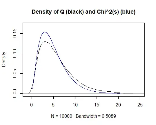
An R simulation below illustrates the performance under $H_0$ and $H_1$ (with $h=4$ and $s=5$). The figure produced under $H_0$ shows that something is not right, however. The test statistic does not have its theoretical distribution in the simulation. I wonder what the problem is, hence a new question "Testing high-order autocorrelations of a low-order MA model with Ljung-Box".

enter image description here


R code:


    # Run only one of the two following lines:
    H0=TRUE ; H1=FALSE # run this for H0
    H0=FALSE; H1=TRUE  # run this for H1
    
    T=1e4 # length of time series
    m=1e4 # number of simulations
    h=4
    s=5
    Qlong=Qshort=rep(NA,m)
    for(i in 1:m){
     set.seed(i)
     if(H0) x=arima.sim(model=list(ma=c(0.6,-0.4,0.2     )),n=T) # under H0
     if(H1) x=arima.sim(model=list(ma=c(0.6,-0.4,0.2,-0.5)),n=T) # under H1
     Qlong [i]=stats::Box.test(x=x,lag=h-1+s,type="Ljung-Box")$statistic
     Qshort[i]=stats::Box.test(x=x,lag=h-1  ,type="Ljung-Box")$statistic
    }
    Q=Qlong-Qshort
    if(H0) Q0=Q # save Q under H0 for later analysis
    if(H1) Q1=Q # save Q under H1 for later analysis
    
    mean(Q) # should be s
    var (Q) # should be 2*s
    
    # Plot kernel density of Q versus theoretical density of Chi^2(s)
    plot(density(Q),xlim=c(-1,25),ylim=c(0,0.17),main="Density of Q (black) and Chi^2(s) (blue)")
    q=qchisq(p=seq(from=0.001,to=0.999,by=0.001),df=s)
    lines(y=dchisq(x=q,df=s),x=q,col="blue")
    
    # Kolmogorov-Smirnov test
    ks.test(Q,"pchisq",s)

Richard Hardy
  • 54,375
  • 10
  • 95
  • 219