Definitions
Recall that a random variable $X$ is a measurable function defined on a probability space $(\Omega,\mathcal{F},\mathbb{P})$ with values in a real vector space $V$. If you would like to focus on concepts and shed the mathematical details, you may think of it as a
consistent way to write numbers on tickets in a box,
as I claimed in an answer at https://stats.stackexchange.com/a/54894. I like this point of view because it beautifully handles complicated generalizations, such as stochastic processes.
Instead of writing a number on each ticket, pick (once and for all) an index space $T$, such as the real numbers (to represent all possible times relative to some starting time) or all natural numbers (to represent discrete time series), or all possible points in space (for a spatial stochastic process). On each ticket $\omega$ there is written an entire real-valued function
$$X(\omega): T\to \mathbb{R}.$$
That's a stochastic process. To sample from it, mix up the tickets thoroughly and pull one out at random with probabilities given by $\mathbb{P}$.
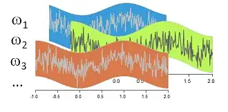
This schematic of a stochastic process $X$ shows parts of three tickets, $\omega_1$, $\omega_2$, and $\omega_3$. On each ticket $\omega$ is displayed a function $X(\omega)$. For any $t$ on the horizontal axis (representing $T$) and any ticket $\omega$ in the box, you can look up the value of $\omega$'s function at $t$ and write it on the ticket: that's the random variable $X(\omega)(t)$.
Equivalent points of view
At the risk of seeming redundant, observe there are three mathematically equivalent ways to view $X$:
A random function $$X(\omega): T \to \mathbb{R}.$$
A random variable whose tickets are time-stamped outcomes in $\Omega$ $$X:T \times \Omega \to \mathbb{R};\quad X(t, \omega) = X(\omega)(t).$$
This is rather a formal equivalence, without a nice tickets-in-box interpretation.
An indexed set of random variables $$X_t: \Omega \to \mathbb{R};\quad X_t(\omega) = X(\omega)(t).$$
To sample from any $X_t$, pick a random ticket $\omega$ from the box and--ignoring the rest of the function $X$--just read its value at $t$.
Neither the sample space $\Omega$ nor the underlying probability measure $\mathbb{P}:\mathcal{F}\to\mathbb{R}$ need to change at all in any of these points of view.
Another approach
To work with a stochastic process, we can often reduce our considerations to finite subsets of $T$. If you fix one $t\in T$, and write the particular value $X(\omega)(t)$ on each ticket, you have--obviously--a random variable. Its name is $X_t$. Formally,
$$X_t(\omega) = X(\omega)(t).$$
If you fix two indexes $s, t\in T$, then you can write the ordered pair $(X(\omega)(s), X(\omega)(t))$ on each ticket $\omega$. This is a bivariate random variable, writen $(X_s, X_t)$. It can be studied like any other bivariate random variable. It has an obvious relationship to the preceding univariate variables $X_t$ and $X_s$: they are its marginals.
You can go further and consider any finite sequence of indexes $\mathcal{T}=(t_1, t_2, \ldots, t_n)$, and similarly define an $n$-variate random variable
$$X_\mathcal{T}(\omega) = (X(\omega)(t_1), X(\omega)(t_2), \ldots, X(\omega)(t_n)).$$
All these multivariate random variables are obviously interconnected. For example, if we re-order the $t_i$ we get another, distinct, random variable--but it's really the "same" random variable with its values re-ordered. And if we simply ignore some of the indexes, we get a kind of generalized marginal distribution, in the same way that $X_s$ is related to $(X_s, X_t)$.
The Kolmogorov Extension Theorem asserts that such a "consistent" family of multivariate random variables, indexed by finite subsets of $T$, is the same thing as the original stochastic process. In other words,
A stochastic process is a consistent family of multivariate radom variables $X_\mathcal{T}$.
Afterward
The Kolmogorov Extension Theorem explains why in much of the literature you will see a focus on analyzing such families, especially for small $n$ (usually $n=1$ and $n=2$). Many kinds of stochastic processes are characterized in terms of them. For instance, in a stationary process a group of transformations $G$ operates transitively on $T$ without changing the distributions of $X_\mathcal{T}$. Specifically, for any $g\in G$ and $\mathcal{T}\subset T$, let $$g(\mathcal{T}) = \{g(t)\,|\, g\in \mathcal{T}\}$$ be the image of $\mathcal{T}$. Then $X_\mathcal{T}$ and $X_{g(\mathcal{T})}$ must have the same (multivariate) distribution. The commonest example is $T=\mathbb{R}$ and $G$ is the group of translations $\{t\to t+g\,|\, g\in\mathbb{R}\}$.
A process is second-order stationary when this invariance relationship is necessarily true for subsets $\mathcal{T}$ having just one or two elements, but perhaps not true for larger subsets. Assuming second-order stationarity means we can focus analysis on the univariate and bivariate distributions determined by $X$ and we don't have to worry about the origin of the "times" $T$.