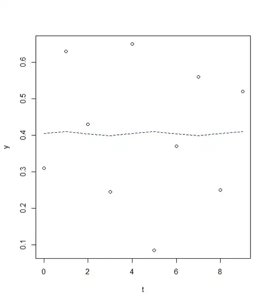
I acquired data (motor adaptation =y in function of delays =t ) which I expect to look like a sine wave. I am trying (1) to fit a sine curve in my data and (2)to estimate the best model/parameters. I read several posts here here here but I am sill struggling.
1) First I tried to use lm
CODE
t<-c(0, 1, 2, 3, 4, 5, 6, 7, 8, 9)
  y<-c(0.310 ,0.630 ,0.430 ,0.245, 0.650 ,0.085 ,0.370, 0.560 ,0.250, 0.520)
reslm <- lm(y ~ sin(pi/2*t)+ cos(pi/2*t)) #my period is supposed to be 4, so period equals to pi/2
summary(reslm)
rg<-(max(y)-min(y)/2)
plot(y~t)
lines(fitted(reslm)~t,col=4,lty=2)
OUTPUT
lm(formula = y ~ sin(pi/2 * t) + cos(pi/2 * t))

Residuals:
     Min       1Q   Median       3Q      Max
-0.32450 -0.13956 -0.00325  0.14819  0.24450

Coefficients:
              Estimate Std. Error t value Pr(>|t|)
(Intercept)   0.404375   0.067993   5.947 0.000572 ***
sin(pi/2 * t) 0.005125   0.095190   0.054 0.958567
cos(pi/2 * t) 0.001125   0.095190   0.012 0.990900
---
Signif. codes:  0 ‘***’ 0.001 ‘**’ 0.01 ‘*’ 0.05 ‘.’ 0.1 ‘ ’ 1

Residual standard error: 0.2107 on 7 degrees of freedom
Multiple R-squared:  0.0004303, Adjusted R-squared:  -0.2852
F-statistic: 0.001507 on 2 and 7 DF,  p-value: 0.998
GRAPH
QUESTIONS
-I am super confused, how can I change the amplitude as well as the pahse shift?
-How can I improve my fit using this methods?
2) Then I tried to use nls
using the equation y(t) = Asin(Omegat + Phi) + C where A is the amplitude, Omega the period, Phi the phase shift and C the midline.
CODE
t<-c(0, 1, 2, 3, 4, 5, 6, 7, 8, 9)
y<-c(0.310 ,0.630 ,0.430 ,0.245, 0.650 ,0.085 ,0.370, 0.560 ,0.250, 0.520)

A<- (max(y)-min(y)/2)
C<-((max(y)+min(y))/2)

res1<- nls(y ~ A*sin(omega*t+phi)+C, data=data.frame(t,y), start=list(A=A,omega=pi/2,phi=0,C=C))
summary(res1)
co <- coef(res1)
resid(res1)
sum(resid(res1)^2)
fit <- function(x, a, b, c, d) {a*sin(b*x+c)+d}
# Plot result
plot(x=t, y=y)
curve(fit(x, a=co["A"], b=co["omega"], c=co["phi"], d=co["C"]), add=TRUE ,lwd=2, col="steelblue")
OUTPUT
Formula: y ~ A * sin(omega * t + phi) + C

Parameters:
       Estimate Std. Error t value Pr(>|t|)
A       0.21956    0.03982   5.513   0.0015 **
omega   2.28525    0.07410  30.841 7.72e-08 ***
phi   -32.57364    0.40375 -80.678 2.44e-10 ***
C       0.41146    0.02926  14.061 8.07e-06 ***
---
Signif. codes:  0 ‘***’ 0.001 ‘**’ 0.01 ‘*’ 0.05 ‘.’ 0.1 ‘ ’ 1

Residual standard error: 0.09145 on 6 degrees of freedom

Number of iterations to convergence: 18
Achieved convergence tolerance: 9.705e-06
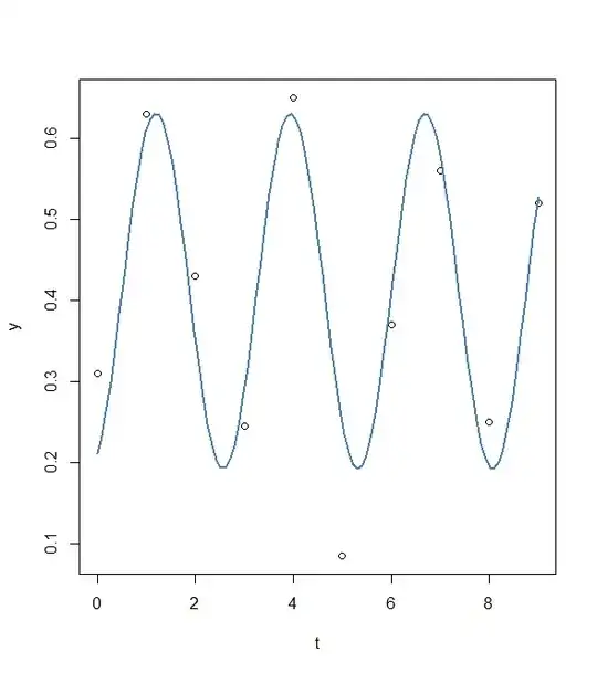
GRAPH
QUESTIONS
-This methods seems working a bit better. But how can I improve the fit using this methods? I tried to change some parameters manually but for example to change phase shift (phi) does not do much or lead to an error ( see part 3).
3) Then I tried to use nls and nsl2, in order to tune my model
CODE
###nls2
t<-c(0, 1, 2, 3, 4, 5, 6, 7, 8, 9)
y<-c(0.310 ,0.630 ,0.430 ,0.245, 0.650 ,0.085 ,0.370, 0.560 ,0.250, 0.520)
A <- (max(y)-min(y)/2)
C<-((max(y)+min(y))/2)
pp <- expand.grid(omega=(c(2.094395, 1.570796,  1.256637)), phi=(-1:1), A=A, C=C) # omega = 2*pi/3, pi/2 , 2*pi/5
View(pp)
pp1<-data.frame(pp)
res2<- nls2(y ~ A*sin(omega*t+phi)+C, data=data.frame(t,y), start=pp1,  algorithm = "brute-force")
res2
summary(res2)
co <- coef(res2)
resid(res2)
sum(resid(res2)^2)
fit <- function(x, a, b, c, d) {a*sin(b*x+c)+d}
# Plot result
plot(x=t, y=y)
curve(fit(x, a=co["A"], b=co["omega"], c=co["phi"], d=co["C"]), add=TRUE ,lwd=2, col="steelblue")

#optimisation
res3<-nls2(y ~ A*sin(omega*t+phi)+C, start = res2)
res3
summary(res3)
co3 <- coef(res3)
resid(res3)
sum(resid(res3)^2)
fit <- function(x, a, b, c, d) {a*sin(b*x+c)+d}
# Plot result
plot(x=t, y=y)
curve(fit(x, a=co3["A"], b=co["omega"], c=co3["phi"], d=co3["C"]), add=TRUE ,lwd=2, col="steelblue")
OUTPUT
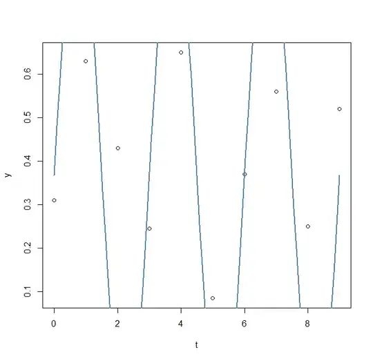
first attempt ( nls2 model1)

model: y ~ A * sin(omega * t + phi) + C
   data: data.frame(t, y)
 omega    phi      A      C
2.0944 0.0000 0.6075 0.3675
 residual sum-of-squares: 0.8545

Number of iterations to convergence: 9
Achieved convergence tolerance: NA
> summary(res2)

Formula: y ~ A * sin(omega * t + phi) + C

Parameters:
      Estimate Std. Error t value Pr(>|t|)
omega  2.09440    0.08453  24.776 2.84e-07 ***
phi    0.00000    0.46494   0.000   1.0000
A      0.60750    0.17851   3.403   0.0144 *
C      0.36750    0.12044   3.051   0.0225 *
---
Signif. codes:  0 ‘***’ 0.001 ‘**’ 0.01 ‘*’ 0.05 ‘.’ 0.1 ‘ ’ 1

Residual standard error: 0.3774 on 6 degrees of freedom

Number of iterations to convergence: 9
Achieved convergence tolerance: NA
GRAPH
Second attempt ( nls2 model2)
Nonlinear regression model
  model: y ~ A * sin(omega * t + phi) + C
   data: <environment>
  omega     phi       A       C
 2.2852 -1.1577  0.2196  0.4115
 residual sum-of-squares: 0.05018

Number of iterations to convergence: 12
Achieved convergence tolerance: 8.075e-06
> summary(res3)

Formula: y ~ A * sin(omega * t + phi) + C

Parameters:
      Estimate Std. Error t value Pr(>|t|)
omega  2.28524    0.07410  30.841 7.72e-08 ***
phi   -1.15769    0.40375  -2.867   0.0285 *
A      0.21956    0.03982   5.513   0.0015 **
C      0.41146    0.02926  14.061 8.07e-06 ***
---
Signif. codes:  0 ‘***’ 0.001 ‘**’ 0.01 ‘*’ 0.05 ‘.’ 0.1 ‘ ’ 1

Residual standard error: 0.09145 on 6 degrees of freedom

Number of iterations to convergence: 12
Achieved convergence tolerance: 8.075e-06
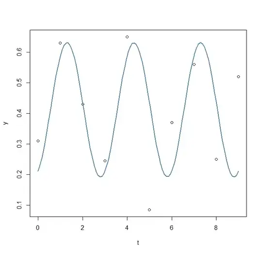
GRAPH
QUESTIONS
-So here it seems I misunderstood what nls2 was doing as I am finding exaclty the same results as part 2... I still do not know which parameters are the best ... How can I do this?
4) Then I tried to use nls, in order to tune my model by looping through several parameters
CODE
t<-c(0, 1, 2, 3, 4, 5, 6, 7, 8, 9)
y<-c(0.310 ,0.630 ,0.430 ,0.245, 0.650 ,0.085 ,0.370, 0.560 ,0.250, 0.520)
A <- (max(y)-min(y)/2)
C<-((max(y)+min(y))/2)
pp <- expand.grid(omega=(c(2.094395, 1.570796,  1.256637)), phi=(-1:1), A=A, C=C) # omega = 2*pi/3, pi/2 , 2*pi/5
#View(pp)

fit_AIC<- vector()
fit_BIC<- vector()

coef_A<- vector()
coef_ome<- vector()
coef_phi<- vector()
coef_C<- vector()
RSS<-vector()

for (ii in 1:nrow(pp))
{
  res<- nls(y ~ A*sin(omega*t+phi)+C, data=data.frame(t,y), start=list(A=pp$A[ii],omega=pp$omega[ii],phi=pp$phi[ii],C=pp$C[ii]), trace = TRUE)
  fit_AIC[ii]<-AIC(res)
  fit_BIC[ii]<-BIC(res)

  coef_A[ii]<- coef(res)[1]
  coef_ome[ii]<- coef(res)[2]
  coef_phi[ii]<- coef(res)[3]
  coef_C[ii]<- coef(res)[4]
  RSS<-sum(resid(res)^2)

}

results<-data.frame(RSS, fit_AIC,  fit_BIC,  coef_A,  coef_ome,  coef_phi,  coef_C)
View(results)
OUTPUT
I get an error...
1.405742 :   0.607500  2.094395 -1.000000  0.367500
0.1448148 :   0.1563179  2.1441802 -0.9937729  0.4172079

...


0.05018035 :   0.2195573  2.2852482 -1.1577097  0.4114573
2.085664 :  0.607500 1.570796 1.000000 0.367500
0.3104012 :  0.01321257 1.60518024 0.83201816 0.40437498
0.3098916 :   0.0180852  3.0888764 -5.9933691  0.4060743
Error in nls(y ~ A * sin(omega * t + phi) + C, data = data.frame(t, y),  :
  le pas 0.000488281 est devenu inférieur à 'minFactor' de 0.000976562


        RSS    fit_AIC    fit_BIC     coef_A  coef_ome    coef_phi    coef_C
1 0.05018035 -14.568398 -13.055473 0.21955754 2.2852455  -1.1576955 0.4114573
2 0.05018035   2.753153   4.266079 0.07487110 0.8575642   0.2299909 0.3916769
3 0.05018035   2.753153   4.266079 0.07487109 0.8575736   0.2299951 0.3916763
4 0.05018035 -14.568398 -13.055473 0.21955763 2.2852443  -1.1576894 0.4114573
5 0.05018035 -14.568398 -13.055473 0.21955729 2.2852490 -32.5736406 0.4114573
6 0.05018035   2.753153   4.266079 0.07487105 0.8575619   0.2300021 0.3916770
7 0.05018035 -14.568398 -13.055473 0.21955735 2.2852482  -1.1577097 0.4114573
QUESTION
-So this error seems to be because my initial parameters are wrong. Is this correct? But how can I estimate the best parameters if the majority of parameters do not work?
-Also, I do not understand why the RSS is always the same despite different parameters
-And why do I observe only 2 different AIC and 2 different BIC while the models are different?
Any kind of help would much appreciated, thanks


