4

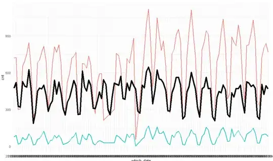
At a news agency, I want to understand whether the number of breaking news infuence the number of citations other media make relative to the news agency.

I do not measure citations of exact news, but only numbers per day totalling to the agency.

enter image description here

The red line stands for regular news, green line is the number of breaking news, and the thick black is the number of citations.

I know the number of news articles where the media mention the news agency (cite_cnt) daily. I also know the number of regular news (news_cnt) and breaking news (flash_cnt) that the news agency made daily.

I build this linear model:

tass_lm <-
     lm(
          cite_cnt ~ news_cnt + flash_cnt
          , dat_tass_cast
     )

summary(tass_lm)


Call:
lm(formula = cite_cnt ~ news_cnt + flash_cnt, data = dat_tass_cast)

Residuals:
     Min       1Q   Median       3Q      Max 
-137.316  -42.530    0.271   32.947  228.625 

Coefficients:
             Estimate Std. Error t value Pr(>|t|)    
(Intercept) 276.37487   17.96854  15.381  < 2e-16 ***
news_cnt      0.09829    0.06547   1.501  0.13595    
flash_cnt     1.39011    0.42608   3.263  0.00145 ** 
---
Signif. codes:  0 ‘***’ 0.001 ‘**’ 0.01 ‘*’ 0.05 ‘.’ 0.1 ‘ ’ 1

Residual standard error: 68.63 on 117 degrees of freedom
Multiple R-squared:  0.6066,    Adjusted R-squared:  0.5998 
F-statistic: 90.19 on 2 and 117 DF,  p-value: < 2.2e-16

To my surprise I found that the number of breaking news is significantly linked to the number of citations. For other news agencies I have the data from, this coefficient is not significant.

So, on top of average level and influence of the regular, I see that breaking news relates to higher number of citations.

Q: I am prone to conclude that 1) breaking news matter a lot if we want more citations. 2) (this is my main question) increasing the number of breaking news will increase citation number if all other factors (including those out of scope) do not change. Is such a causal reference vaild in this case?

Update:

tass_lm <-
     lm(
          cite_cnt ~ as.factor(dweek) + news_cnt + flash_cnt
          , dat_tass_cast
     )

summary(tass_lm)


Call:
lm(formula = cite_cnt ~ as.factor(dweek) + news_cnt + flash_cnt, 
    data = dat_tass_cast)

Residuals:
     Min       1Q   Median       3Q      Max 
-110.880  -37.185   -0.297   30.907  117.174 

Coefficients:
                   Estimate Std. Error t value Pr(>|t|)    
(Intercept)       283.66023   15.67226  18.100  < 2e-16 ***
as.factor(dweek)2 146.71450   19.30685   7.599 1.02e-11 ***
as.factor(dweek)3 163.97176   20.55983   7.975 1.49e-12 ***
as.factor(dweek)4 162.46087   21.41195   7.587 1.08e-11 ***
as.factor(dweek)5 170.88246   21.52676   7.938 1.80e-12 ***
as.factor(dweek)6 164.23197   19.08878   8.604 5.70e-14 ***
as.factor(dweek)7   6.24548   16.87997   0.370    0.712    
news_cnt           -0.12054    0.05378  -2.241    0.027 *  
flash_cnt           1.56664    0.32715   4.789 5.22e-06 ***
---
Signif. codes:  0 ‘***’ 0.001 ‘**’ 0.01 ‘*’ 0.05 ‘.’ 0.1 ‘ ’ 1

Residual standard error: 49.21 on 111 degrees of freedom
Multiple R-squared:  0.8081,    Adjusted R-squared:  0.7943 
F-statistic: 58.43 on 8 and 111 DF,  p-value: < 2.2e-16

Update 2 (GLM):

Using GLM with the Possion family resulted in even higer t-statistic for the breaking news counts.

tass_glm <-
     glm(
          cite_cnt ~ as.factor(dweek) + news_cnt + flash_cnt
          , dat_tass_cast
          , family = poisson(link = "log")
     )

summary(tass_glm)

Call:
glm(formula = cite_cnt ~ as.factor(dweek) + news_cnt + flash_cnt, 
    family = poisson(link = "log"), data = dat_tass_cast)

Deviance Residuals: 
    Min       1Q   Median       3Q      Max  
-6.0270  -1.8957  -0.0114   1.5932   6.7059  

Coefficients:
                    Estimate Std. Error z value Pr(>|z|)    
(Intercept)        5.647e+00  1.754e-02 322.026  < 2e-16 ***
as.factor(dweek)2  4.148e-01  2.046e-02  20.277  < 2e-16 ***
as.factor(dweek)3  4.535e-01  2.152e-02  21.073  < 2e-16 ***
as.factor(dweek)4  4.468e-01  2.213e-02  20.189  < 2e-16 ***
as.factor(dweek)5  4.620e-01  2.211e-02  20.894  < 2e-16 ***
as.factor(dweek)6  4.539e-01  2.009e-02  22.590  < 2e-16 ***
as.factor(dweek)7  2.035e-02  2.023e-02   1.006    0.314    
news_cnt          -2.474e-04  5.234e-05  -4.727 2.28e-06 ***
flash_cnt          3.290e-03  3.094e-04  10.632  < 2e-16 ***
---
Signif. codes:  0 ‘***’ 0.001 ‘**’ 0.01 ‘*’ 0.05 ‘.’ 0.1 ‘ ’ 1

(Dispersion parameter for poisson family taken to be 1)

    Null deviance: 3462.96  on 119  degrees of freedom
Residual deviance:  676.84  on 111  degrees of freedom
AIC: 1639.5

Number of Fisher Scoring iterations: 4
Alexey Burnakov
  • 2,469
  • 11
  • 23
  • 2
    My suggestion is to separately model work days from non-work days, that is, weekdays from weekends. The variation due to lower weekend numbers is quite large and might be disguising the actual trends. – James Phillips Nov 01 '19 at 13:45
  • 1
    You can't draw conclusions of causal relationships based on an observational study. In addition, have you considered the model assumptions? Citation counts are likely skewed and would fit better in a discrete GLM. Moreover, I think the problem is more complex: The effect of one event (breaking news) on a possibly delayed other event (citations) makes more sense in the context of a distributed lag model. – Frans Rodenburg Nov 01 '19 at 13:50
  • 1
    *For other news agencies I have the data from, this coefficient is not significant.* ... I think that there might be some other variable that might be at play here. Is this particular news agency different kind than the others that you mention? If so, how and what other variables can be included in the model. – naive Nov 01 '19 at 13:51
  • @JamesPhillips, I tried to accomodate for the week day based variance by updating my model (in first post), and I still see that breaking news coefficient is significant. – Alexey Burnakov Nov 01 '19 at 14:25
  • @FransRodenburg, as to lag point, yes, I know exactly how much lag a citation can take based on other studies I have made, but it is mostly inside one day, so I cannot take daily lags, which will be mostly misleading. What I can try is to model citations for each exact breaking news to understand how much agencies compare in terms of the mean citation rate per news. I will try now discrete GLM, thank you. – Alexey Burnakov Nov 01 '19 at 14:30
  • @naive, Sure, other factors exist. They can be distribution of topics, probability of brekaing news over topics, distribution of news delivery time inside a day, and more. But the first thing I was asked to investigate is whether breaking news are associated with citations, without further details. – Alexey Burnakov Nov 01 '19 at 14:41
  • @FransRodenburg, you said "You can't draw conclusions of causal relationships based on an observational study." This is the answer I wanted, but... What is the formulation most appropriate here? Is this a good wording? "I observe that the citation number for the whole agency is significantly affected by breaking news number, taking into consideration the factors of regular news number and week days (and hence managing breaking news rates/numers can influence the citation rate)"? I am going to report to layman audience (not stats knowledge at all). – Alexey Burnakov Nov 01 '19 at 14:57

3 Answers3

3

People in the causal inference literature would reject a causal inference from these results, because these analyses are at risk of endogeneity--an unobserved common cause for your predictors and your dependent variable. Elwert's (2013) chapter is a gentle introduction to one strand of the causal inference literature. The point of this strand is that you need instrumental variables (which cause predictors but not the outcome variable) in order to rule out endogeneity as a confound.

But there are other approaches, which aim to strengthen the case for a causal interpretation. Still, regression alone does not make the case. It is justified to say that the regression evidence is not inconsistent with the proposed interpretation.

Ed Rigdon
  • 1,341
  • 4
  • 11
  • Thank you. I know the endogeneity issue, and I knew it was in place, but I was not sure the extent of its influence. I tried to grab the possible factors which make sense intuitively and some of them worked. However, I made a point when presenting these results that I could not look into all possible major factors just because I don't have access to them technically. So we agreed that a small experiment based on causation could be made. It is also very hard to explain the concept to non-tech guys... I will read the paper, many thanks. – Alexey Burnakov Dec 27 '19 at 13:17
2

Look at http://www.autobox.com/pdfs/regvsbox-old.pdf as you are analyzing time series data that has autocorrelation possibly (probably !) vitiating your conclusions. Did you verify that your final model's residuals were free of structure i.e. were white noise and uncorrelated with lags of your predictor series suggesting sufficiency?

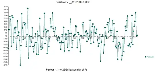
I will start by analyzing the 173 model residuals that you posted in order to assess that they are free of structure , both stochastic and deterministic . The plot of the data enter image description herenot only reveals anomalies but can hide/obfuscate latent deterministic structure like day-of-the-week effects.

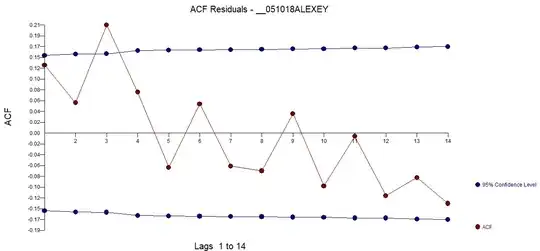
The ACF of these 173 residuals is here enter image description here suggesting randomness BUT that is only true if there are no latent deterministic factors (pulses and seasonal pulses ) present in the data which would lead to an underestimation of the ACF as the variance of the errors is enlarged (over-estimated).

Determining parameters (p, d, q) for ARIMA modeling discusses Prof. Keith Ord's "Alice in Wonderland effect" .

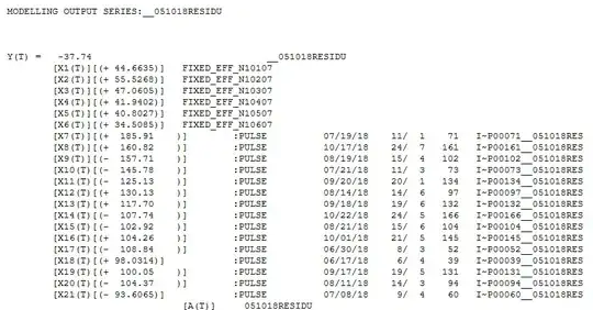
A routine analysis suggests 6 very strong seasonal pulses reflecting omitted day-pf-the week effects shown here enter image description here and here enter image description here . The idea that latent deterministic effects provide down-sized estimates of the ACF is the "small print" that many ignore but not all !

Thus there is sufficient information now that the residuals are not free-of-structure thus model conclusions may be flawed. After clarification from the OP about his original data , I will follow this up .

AFTER RECEIPT OF ORIGINAL DATA: enter image description here and here enter image description here . The analysis showed that X2 was not significant ( NOT CLOSE TO BEING SIGNIFICANT ) with daily indicators being detected AND two counter-weighting level shifts .

The model is here enter image description here

The residual plot here enter image description here with an ACF here enter image description here

The Forecast Plot is here (using ARIMA forecasts for X1) enter image description here

enter image description here

IrishStat
  • 27,906
  • 5
  • 29
  • 55
  • Hello. Thank you. This is a good point. I will check for residual serial dependencies. However, I did some study of the residuals (updated my answer), but not with this rigour. – Alexey Burnakov Dec 27 '19 at 13:20
  • 1
    If you wish to share your data , I will try and provide some guidance. – IrishStat Dec 27 '19 at 13:22
  • I uploaded residual data to my github: https://raw.githubusercontent.com/alexmosc/ds_lectures/master/diff_lm_res.csv If you have time to look at them, I would be grateful. – Alexey Burnakov Dec 27 '19 at 13:42
  • 1
    please add the original data matrix – IrishStat Dec 27 '19 at 13:43
  • I uploaded design matrix: https://raw.githubusercontent.com/alexmosc/ds_lectures/master/diff_lm_dataset.csv. My model was designed like this: {lm( ria_tass_cite_diff ~ as.factor(which_month) + ria_tass_top_msg_diff + ria_tass_bottom_msg_diff + ria_tass_top_flash_diff + ria_tass_bottom_flash_diff , dt_final )} – Alexey Burnakov Dec 27 '19 at 13:53
  • 1
    Your 5 time series are a collection of observed and derived (by your assumption) . Please tell me , the pointer for the Y variable and the pointers for the 2 X variables that were originally observed . – IrishStat Dec 27 '19 at 14:06
  • My Y variable is "ria_tass_cite_diff". Variables "ria_tass_top_msg_diff","ria_tass_bottom_msg_diff","ria_tass_top_flash_diff","ria_tass_bottom_flash_diff" are actually observed independent variables. **The next 2 variables are of most interest:** "ria_tass_top_flash_diff","ria_tass_bottom_flash_diff" (they are breaking news count differences in high and low interest news topics). – Alexey Burnakov Dec 27 '19 at 14:12
  • 1
    I am confused , please post the data without any differences or lags that you injected. Please post three naturally observed series ... a Y and 2 X's . – IrishStat Dec 27 '19 at 14:35
  • Ahh, I see what you mean. I did not differenced the data in a time-lag sense. The data you see are the daily deltas between two news agencies, as: RIA Citaions - TASS Citations = ria_tass_cite_diff, at day 2019-10-01. So these are raw data. My hypothesis is if the delta in citations is explained by the deltas in other timseries: **ria_tass_top_msg_diff","ria_tass_bottom_msg_diff","ria_tass_top_flash_diff","ria_tass_bottom_flash_diff"**, and they are not differenced either. **is it OK?** – Alexey Burnakov Dec 27 '19 at 14:40
  • Originally in my question I started with these data: https://raw.githubusercontent.com/alexmosc/ds_lectures/master/original_diff_lm_dataset.csv. Here I modeled **Y ~ x2 + x1**. I was interested in x2 mostly, accomodating for the presence of x1. These are raw daily counts (not deltas) for just 1 news agency. – Alexey Burnakov Dec 27 '19 at 14:53
  • Thank you, Sir. So my model is flawed, I take it as a guideance for next research. Thanks for your analysis. Having a glass of Jameson Old Oak for you. – Alexey Burnakov Dec 28 '19 at 12:16
  • 1
    please accept my answer and also upvote it . How did you know I prefer J ? – IrishStat Dec 28 '19 at 12:36
  • I did it, although another was already accepted. We spoke a year ago in another topic and we discussed J – Alexey Burnakov Dec 28 '19 at 13:33
  • 1
    Good memory . I am glad I could help you ... – IrishStat Dec 28 '19 at 20:24
  • https://stats.stackexchange.com/questions/311492/forecasting-next-12-months-based-on-previous-data-using-r/311511#comment591868_311511 – Alexey Burnakov Dec 31 '19 at 09:52
1

So I finally took my time to try to answer the question about casuality in my data.

First off, I get the difference of all metrics (both indeoendent and dependent) for two major news agencies, us and a competitor. This makes data more stable, somewhat stationary.

Dependent variable (difference between two agencies' citation number):

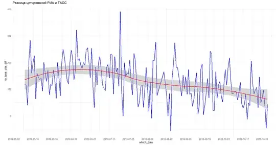
enter image description here

So I formulate my hypothesis as this: can we say that the difference in the number of breaking news influences the number of citations of the agency.

In the next step I insert some factors I think are important hidden explanatory variables: month of the year, regular news, and all the news were divided into two categories: ones belonging to low-interest topics, and ones belonding to high-interest topics.

It turned out that:

ria_tass_top_flash_diff

the independent variable of the difference between the high-interest breaking news shows 2.7 t-statistic, while the low-interest breaking news are not significant. This is in leu with the intuition.

I also made a contrast study, by means of comparing nested models of increasing complecity, and the f-statistic was likewise high of this variable.

My final phrasing for this study was that: "

There is an (optimistic) indication that increasing breaking number in high-interest topics can increase the citation number, given that all influential factors were accounted for in the final model.

"

However, there is also a realistic note saying we could not take into account all possible factors, which means the coefficient estimate 0.799 is an upper bounded forecast, while the real effect can be zero.

Final model:

enter image description here

Residuals:

enter image description here

Alexey Burnakov
  • 2,469
  • 11
  • 23
  • you basically contradict your statement In your footnote. you should reword your quote *...citation number,* **noting** *that all influential factors were* **not** *accounted for in the final model.* should also verify that your models forecasts are accurate – probabilityislogic Dec 27 '19 at 13:41
  • @probabilityislogic, ahh, yes, I know what you meant. This is (in my version of English) the same statement. I said we optimistically found that the causal relation was there IF all hidden factors were also there. I meant there was no room for more factors. I can also say that I note that not all influential factors were accounted for. – Alexey Burnakov Dec 27 '19 at 13:45