In general, dig into an advanced time series analysis textbook (introductory books will usually direct you to just trust your software), like Time Series Analysis by Box, Jenkins & Reinsel. You may also find details on the Box-Jenkins procedure by googling. Note that there are other approaches than Box-Jenkins, e.g., AIC-based ones.
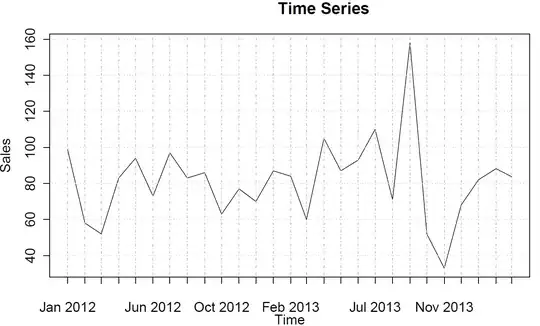
In R, you first convert your data into a ts (time series) object and tell R that the frequency is 12 (monthly data):
require(forecast)
sales <- ts(c(99, 58, 52, 83, 94, 73, 97, 83, 86, 63, 77, 70, 87, 84, 60, 105, 87, 93, 110, 71, 158, 52, 33, 68, 82, 88, 84),frequency=12)
You can plot the (partial) autocorrelation functions:
acf(sales)
pacf(sales)
These don't suggest any AR or MA behavior.
Then you fit a model and inspect it:
model <- auto.arima(sales)
model
See ?auto.arima for help. As we see, auto.arima chooses a simple (0,0,0) model, since it sees neither trend nor seasonality nor AR or MA in your data. Finally, you can forecast and plot the time series and forecast:
plot(forecast(model))
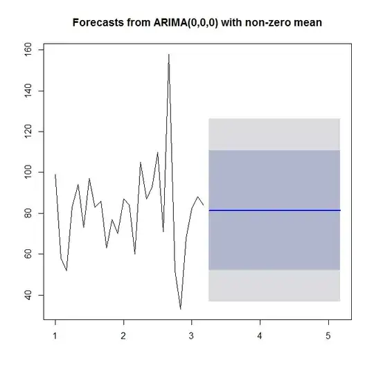
Look at ?forecast.Arima (note the capital A!).
This free online textbook is a great introduction to time series analysis and forecasting using R. Very much recommended.