The Anderson-Darling test is a good test--but it has to be correctly applied and, as in most distributional tests, there is a subtle pitfall. Many analysts have fallen for it.
Distributional tests are Cinderella tests. In the fairy tale, the prince's men searched for a mysterious princess by comparing the feet of young ladies to the glass slipper Cinderella had left behind as she fled the ball. Any young lady whose foot fit the slipper would be a "significant" match to the slipper. This worked because the slipper had a specific shape, length, and width and few feet in the realm would likely fit it.

Imagine a twist on this fairy tale in which Cinderella's ugly stepsisters got wind of the search. Before the prince's men arrived, the stepsisters visited Ye Olde Paylesse Glasse Slipper Store and chose a slipper off the rack to match the width and length of the eldest sister's foot. Because glass slippers are not malleable and this one was not specifically tailored to the foot, it was not perfect--but at least the shoe fit.
Returning to their home just as the prince's men arrived, the older sister distracted the men while the younger surreptitiously substituted the slipper she had just purchased for the one brought by the men. When the men offered this slipper to the older sister, they were astonished that it fit her warty foot. Nevertheless, because she had passed the test she was promptly brought before the prince.
I hope the prince, like you, was sufficiently sharp-eyed and clever to recognize that the ugly lady brought before him could not possibly be the same beautiful girl he had danced with at the ball. He wondered, though, how the slipper could possibly fit her foot.
That is precisely what this question asks: how can the goftest version of the A-D test seem like the dataset is such a good match to the Normal distribution "slipper" while the nortest version indicates it is not? The answer is that the goftest version was offered a distribution constructed to match the data while the nortest version anticipates that subterfuge and compensates accordingly, as did the prince.
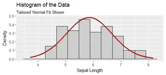
The goftest version of the Anderson-Darling test asks you to provide the glass slipper in the form of "distributional parameters," which are perfect analogs of length and width. This version compares your distribution to the data and reports how well it fits. As applied in the question, though, the distributional parameters were tailored to the data: they were estimated from them. In exactly the same way the ugly stepsister's foot turned out to be a good match to the slipper, so will these data appear to be a good match to a Normal distribution, even when they are (to any sufficiently sharp-eyed prince) obviously non-Normal.
The nortest version assumes you are going to cheat in this way and it automatically compensates for that. It reports the same degree of fit--that's why the two A-D statistics of 0.8892 shown in the question are the same--but it assesses its goodness in a manner that compensates for the cheating.
It is possible to adjust the goftest version to produce a correct p-value. One way is through simulation: by repeatedly offering samples from a Normal distribution to the test, we can discover the distribution of its test statistic (or, equivalently, the distribution of the p-values it assigns to that statistic). Only p-values that are extremely low relative to this null distribution should count as evidence that the shoe fits.
Here is a histogram of 100,000 iterations of this simulation.
P-values are supposed to have a uniform distribution (when the null hypothesis is true). The histogram would be almost level. This distribution is decidedly non-uniform.
The vertical line is at $0.42,$ the p-value reported for the original data. The values smaller than it are shown in red as "extreme." Only $0.0223$ of them are this extreme. (The first three decimal places of this number should be correct.) This is the correct p-value for this test. It is in close agreement with the value of $0.0251$ reported by nortest. (In this case, because I performed such a large simulation, the simulated p-value should be considered more accurate than the computed p-value.)
The R code that produced the simulation and the figure is reproduced below, but with the simulation size set to 1,000 rather than 100,000 so that it will execute in less than one second.
library(ggplot2)
x = iris$Sepal.Length
p.value <- goftest::ad.test(x, "pnorm", mean = mean(x), sd = sd(x))$p.value
#
# Simulation study.
#
mu <- mean(x)
sigma <- sd(x)
sim <- replicate(1e3, {
  x.sim <- rnorm(length(x), mu, sigma)
  goftest::ad.test(x.sim, "pnorm", mean = mean(x.sim), sd = sd(x.sim))$p.value
})

p.value.corrected <- mean(sim <= p.value)
message("Corrected p-value is ", p.value.corrected,
        " +/- ", signif(2 * sd(sim <= p.value) / sqrt(length(sim)), 2))
#
# Display the p-value distribution.
#
X <- data.frame(p.value=sim, Status=ifelse(sim <= p.value, "Extreme", "Not extreme"))
ggplot(X, aes(p.value)) +
  xlab("goftest::ad.test p-value") + ylab("Count") +
  geom_histogram(aes(fill=Status), binwidth=0.05, boundary=0, alpha=0.65) +
  geom_vline(xintercept=p.value, color="#404040", size=1) +
  ggtitle("A-D 'p-values' for Simulated Normal Data",
          "`goftest` calculations")


