How to determine significant principal components using bootstrapping or Monte Carlo approach?

Question

I am interested in determining the number of significant patterns coming out of a Principal Component Analysis (PCA) or Empirical Orthogonal Function (EOF) Analysis. I am particularly interested in applying this method to climate data. The data field is a MxN matrix with M being the time dimension (e.g. days) and N being the spatial dimension (e.g. lon/lat locations). I have read of a possible bootstrap method to determine significant PCs, but have been unable to find a more detailed description. Until now, I have been applying North's Rule of Thumb (North et al., 1982) to determine this cutoff, but I was wondering if a more robust method was available.

As an example:

###Generate data
x <- -10:10
y <- -10:10
grd <- expand.grid(x=x, y=y)

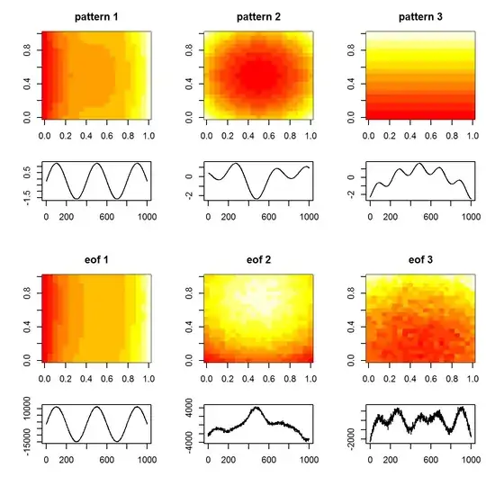
#3 spatial patterns
sp1 <- grd$x^3+grd$y^2
tmp1 <- matrix(sp1, length(x), length(y))
image(x,y,tmp1)

sp2 <- grd$x^2+grd$y^2
tmp2 <- matrix(sp2, length(x), length(y))
image(x,y,tmp2)

sp3 <- 10*grd$y
tmp3 <- matrix(sp3, length(x), length(y))
image(x,y,tmp3)


#3 respective temporal patterns
T <- 1:1000

tp1 <- scale(sin(seq(0,5*pi,,length(T))))
plot(tp1, t="l")

tp2 <- scale(sin(seq(0,3*pi,,length(T))) + cos(seq(1,6*pi,,length(T))))
plot(tp2, t="l")

tp3 <- scale(sin(seq(0,pi,,length(T))) - 0.2*cos(seq(1,10*pi,,length(T))))
plot(tp3, t="l")


#make data field - time series for each spatial grid (spatial pattern multiplied by temporal pattern plus error)
set.seed(1)
F <- as.matrix(tp1) %*% t(as.matrix(sp1)) + 
as.matrix(tp2) %*% t(as.matrix(sp2)) + 
as.matrix(tp3) %*% t(as.matrix(sp3)) +
matrix(rnorm(length(T)*dim(grd)[1], mean=0, sd=200), nrow=length(T), ncol=dim(grd)[1]) # error term

dim(F)
image(F)


###Empirical Orthogonal Function (EOF) Analysis 
#scale field
Fsc <- scale(F, center=TRUE, scale=FALSE)

#make covariance matrix
C <- cov(Fsc)
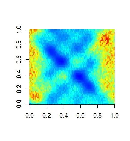
image(C)

#Eigen decomposition
E <- eigen(C)

#EOFs (U) and associated Lambda (L) 
U <- E$vectors
L <- E$values

#projection of data onto EOFs (U) to derive principle components (A)
A <- Fsc %*% U

dim(U)
dim(A)

#plot of top 10 Lambda
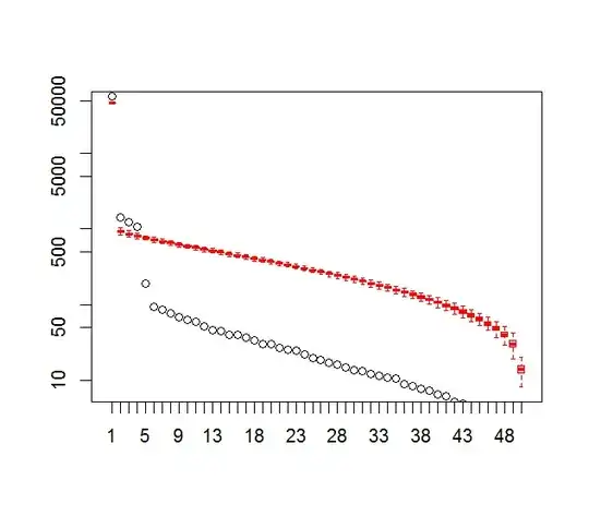
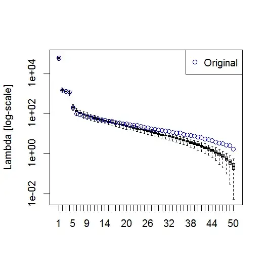
plot(L[1:10], log="y")

#plot of explained variance (explvar, %) by each EOF
explvar <- L/sum(L) * 100
plot(explvar[1:20], log="y")


#plot original patterns versus those identified by EOF
layout(matrix(1:12, nrow=4, ncol=3, byrow=TRUE), widths=c(1,1,1), heights=c(1,0.5,1,0.5))
layout.show(12)

par(mar=c(4,4,3,1))
image(tmp1, main="pattern 1")
image(tmp2, main="pattern 2")
image(tmp3, main="pattern 3")

par(mar=c(4,4,0,1)) 
plot(T, tp1, t="l", xlab="", ylab="")
plot(T, tp2, t="l", xlab="", ylab="")
plot(T, tp3, t="l", xlab="", ylab="")

par(mar=c(4,4,3,1))
image(matrix(U[,1], length(x), length(y)), main="eof 1") 
image(matrix(U[,2], length(x), length(y)), main="eof 2")
image(matrix(U[,3], length(x), length(y)), main="eof 3")

par(mar=c(4,4,0,1)) 
plot(T, A[,1], t="l", xlab="", ylab="")
plot(T, A[,2], t="l", xlab="", ylab="")
plot(T, A[,3], t="l", xlab="", ylab="")

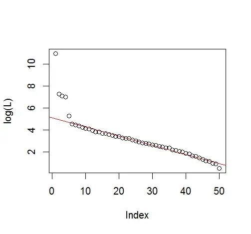
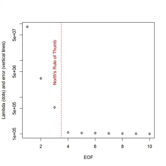
And, here is the method that I have been using to determine PC significance. Basically, the rule of thumb is that the difference between neighboring Lambdas must be greater than their associated error.

###Determine significant EOFs

#North's Rule of Thumb
Lambda_err <- sqrt(2/dim(F)[2])*L
upper.lim <- L+Lambda_err
lower.lim <- L-Lambda_err
NORTHok=0*L
for(i in seq(L)){
    Lambdas <- L
    Lambdas[i] <- NaN
    nearest <- which.min(abs(L[i]-Lambdas))
    if(nearest > i){
        if(lower.lim[i] > upper.lim[nearest]) NORTHok[i] <- 1
    }
    if(nearest < i){
        if(upper.lim[i] < lower.lim[nearest]) NORTHok[i] <- 1
    }
}
n_sig <- min(which(NORTHok==0))-1

plot(L[1:10],log="y", ylab="Lambda (dots) and error (vertical lines)", xlab="EOF")
segments(x0=seq(L), y0=L-Lambda_err, x1=seq(L), y1=L+Lambda_err)
abline(v=n_sig+0.5, col=2, lty=2)
text(x=n_sig, y=mean(L[1:10]), labels="North's Rule of Thumb", srt=90, col=2)

I have found the chapter section by Björnsson and Venegas (1997) on significance tests to be helpful - they refer to three categories of tests, of which the dominant variance-type is probably what I am hoping to use. The refer to a type of Monte Carlo approach of shuffling the time dimension and recomputing the Lambdas over many permutations. von Storch and Zweiers (1999) also refer to the a test that compares the Lambda spectrum to a reference "noise" spectrum. In both cases, I am a bit unsure of how this might be done, and also how the significance test is done given the confidence intervals identified by the permutations.

Thanks for your help.

References: Björnsson, H. and Venegas, S.A. (1997). "A manual for EOF and SVD analyses of climate data", McGill University, CCGCR Report No. 97-1, Montréal, Québec, 52pp. http://andvari.vedur.is/%7Efolk/halldor/PICKUP/eof.pdf

G.R. North, T.L. Bell, R.F. Cahalan, and F.J. Moeng. (1982). Sampling errors in the estimation of empirical orthogonal functions. Mon. Wea. Rev., 110:699–706.

von Storch, H, Zwiers, F.W. (1999). Statistical analysis in climate research. Cambridge University Press.

Answer 1

I am going to try and advance the dialogue here a bit even though this is my question. It's been 6 months since I asked this and unfortunately no complete answers have been given I will try and summarize what I have gathered thus far and see if anyone can elaborate on remaining issues. Please excuse the lengthy answer, but I see no other way...

First, I will demonstrate several approaches using a possibly better synthetic data set. It comes from a paper by Beckers and Rixon (2003) illustrating the use of an algorithm for conducting EOF on gappy data. I have reproduced the algorithm in R if anyone is interested (link).

Synthetic data set:

#color palette
pal <- colorRampPalette(c("blue", "cyan", "yellow", "red"))

#Generate data
m=50
n=100
frac.gaps <- 0.5 # the fraction of data with NaNs
N.S.ratio <- 0.25 # the Noise to Signal ratio for adding noise to data

x <- (seq(m)*2*pi)/m
t <- (seq(n)*2*pi)/n


#True field
Xt <- 
 outer(sin(x), sin(t)) + 
 outer(sin(2.1*x), sin(2.1*t)) + 
 outer(sin(3.1*x), sin(3.1*t)) +
 outer(tanh(x), cos(t)) + 
 outer(tanh(2*x), cos(2.1*t)) + 
 outer(tanh(4*x), cos(0.1*t)) + 
 outer(tanh(2.4*x), cos(1.1*t)) + 
 tanh(outer(x, t, FUN="+")) + 
 tanh(outer(x, 2*t, FUN="+"))

Xt <- t(Xt)
image(Xt, col=pal(100))

#Noise field
set.seed(1)
RAND <- matrix(runif(length(Xt), min=-1, max=1), nrow=nrow(Xt), ncol=ncol(Xt))
R <- RAND * N.S.ratio * Xt

#True field + Noise field
Xp <- Xt + R
image(Xp, col=pal(100))

So, the true data field Xtis comprised of 9 signals and I have added some noise to it to create the observed field Xp, which will be used in the examples below. The EOFs are determined as such:

EOF

#make covariance matrix
C <- t(Xp) %*% Xp #cov(Xp)
image(C)

#Eigen decomposition
E <- svd(C)

#EOFs (U) and associated Lambda (L) 
U <- E$u
L <- E$d

#projection of data onto EOFs (U) to derive principle components (A)
A <- Xp %*% U

Following the example that I used in my original example, I will determine "significant" EOFs via North's rule of thumb.

North's Rule of Thumb

Lambda_err <- sqrt(2/dim(Xp)[2])*L
upper.lim <- L+Lambda_err
lower.lim <- L-Lambda_err
NORTHok=0*L
for(i in seq(L)){
    Lambdas <- L
    Lambdas[i] <- NaN
    nearest <- which.min(abs(L[i]-Lambdas))
    if(nearest > i){
        if(lower.lim[i] > upper.lim[nearest]) NORTHok[i] <- 1
    }
    if(nearest < i){
        if(upper.lim[i] < lower.lim[nearest]) NORTHok[i] <- 1
    }
}
n_sig <- min(which(NORTHok==0))-1
n_sig

plot(L[1:20],log="y", ylab="Lambda (dots) and error (vertical lines)", xlab="EOF")
segments(x0=seq(L), y0=L-Lambda_err, x1=seq(L), y1=L+Lambda_err)
abline(v=n_sig+0.5, col=2, lty=2)
text(x=n_sig, y=mean(L[1:10]), labels="North's Rule of Thumb", srt=90, col=2)

Since the Lambda values of 2:4 are very close to each other in amplitude, these are deemed insignificant by the rule of thumb - i.e. their respective EOF patterns might overlap and mix given their similar amplitudes. This is unfortunate given that we know that 9 signals actually exist in the field.

A more subjective approach is to view the log-transformed Lambda values ("Scree plot") and to then fit a regression to the trailing values. One then can determine visually at what level the lambda values lie above this line:

Scree plot

ntrail <- 35
tail(L, ntrail)
fit <- lm(log(tail(L, ntrail)) ~ seq(length(L)-ntrail+1, length(L)))
plot(log(L))
abline(fit, col=2)

So, the 5 leading EOFs lie above this line. I have tried this example when Xp has no additional noise added and the results reveal all 9 original signals. So, the insignificance of EOFs 6:9 is due to the fact that their amplitude is lower than the noise in the field.

A more objective method is the "Rule N" criteria by Overland and Preisendorfer (1982). There is an implementation within the wq package, which I show below.

Rule N

library(wq)
eofNum(Xp, distr = "normal", reps = 99)

RN <- ruleN(nrow(Xp), ncol(Xp), type = "normal", reps = 99)
RN
eigs <- svd(cov(Xp))$d
plot(eigs, log="y")
lines(RN, col=2, lty=2)

The Rule N identified 4 significant EOFs. Personally, I need to better understand this method; Why is it possible to gauge the level of error based on a random field that does not use the same distribution as that in Xp? One variation on this method would be to resample the data in Xp so that each column is reshuffled randomly. In this way, we ensure that the total variance of the random field is the same as Xp. By resampling many times, we are then able to calculate a baseline error of the decomposition.

Monte Carlo with random field (i.e. Null model comparison)

iter <- 499
LAMBDA <- matrix(NaN, ncol=iter, nrow=dim(Xp)[2])

set.seed(1)
for(i in seq(iter)){
    #i=1

    #random reorganize dimensions of scaled field
    Xp.tmp <- NaN*Xp
    for(j in seq(dim(Xp.tmp)[2])){
        #j=1
        Xp.tmp[,j] <- Xp[,j][sample(nrow(Xp))]
    }

    #make covariance matrix
    C.tmp <- t(Xp.tmp) %*% Xp.tmp #cov(Xp.tmp)

    #SVD decomposition
    E.tmp <- svd(C.tmp)

    #record Lambda (L) 
    LAMBDA[,i] <- E.tmp$d

    print(paste(round(i/iter*100), "%", " completed", sep=""))
}

boxplot(t(LAMBDA), log="y", col=8, border=2, outpch="")
points(L)

Again, 4 EOFs are above the distributions for the random fields. My worry with this approach, and that of Rule N, is that these are not truly addressing the confidence intervals of the Lambda values; e.g. a high first Lambda value will automatically result in a lower amount of variance to be explained by trailing ones. Thus the Lambda calculated from random fields will always have a less steep slope and may result in selecting too few significant EOFs. [NOTE: The eofNum() function assumes that EOFs are calculated from a correlation matrix. This number might be different if using a e.g. a covariance matrix (centered but not scaled data).]

Finally, @tomasz74 mentioned the paper by Babamoradi et al. (2013), which I have had a brief look at. Its very interesting, but seems to be more focused on calculating CI's of EOF loadings and coefficients, rather than Lambda. Nevertheless, I believe that it might be adopted to assess Lambda error using the same methodology. A bootstrap resampling is done of the data field by resampling the rows until a new field is produced. The same row can be resampled more than once, which is a non-parametric approach and one does not need to make assumptions about the distribution of data.

Bootstrap of Lambda values

B <- 40 * nrow(Xp)
LAMBDA <- matrix(NaN, nrow=length(L), ncol=B)
for(b in seq(B)){
    samp.b <- NaN*seq(nrow(Xp))
    for(i in seq(nrow(Xp))){
        samp.b[i] <- sample(nrow(Xp), 1)
    }
    Xp.b  <- Xp[samp.b,]
    C.b  <- t(Xp.b) %*% Xp.b 
    E.b  <- svd(C.b)
    LAMBDA[,b] <- E.b$d
    print(paste(round(b/B*100), "%", " completed", sep=""))
}
boxplot(t(LAMBDA), log="y", col=8, outpch="", ylab="Lambda [log-scale]")
points(L, col=4)
legend("topright", legend=c("Original"), pch=1, col=4)

While this may be a more robust than North's rule of thumb for calculating the error of Lambda values, I believe now that the question of EOF significance comes down to different opinions on what this means. For the North's rule of thumb and bootstrap methods, significance appears to be more based on whether or not teere is overlap between Lambda values. If there is, then these EOFs may be mixed in their signals and not represent "true" patterns. On the other hand, these two EOFs may describe a significant amount of variance (as compared to the decomposition of a random field - e.g. Rule N). So if one is interested in filtering out noise (i.e via EOF truncation) then Rule N would be sufficient. If one is interested in determining real patterns in a data set, then the more stringent criteria of Lambda overlap may be more robust.

Again, I am not an expert in these issues, so I am still hoping that someone with more experience can add to this explanation.

References:

Beckers, Jean-Marie, and M. Rixen. "EOF Calculations and Data Filling from Incomplete Oceanographic Datasets." Journal of Atmospheric and Oceanic Technology 20.12 (2003): 1839-1856.

Overland, J., and R. Preisendorfer, A significance test for principal components applied to a cyclone climatology, Mon. Wea. Rev., 110, 1-4, 1982.