Interpreting 2D correspondence analysis plots (Part II)

Question

I'd like to ensure that I understand the process correctly. This is a follow-up question to Interpreting 2D correspondence analysis plots

library(reshape) 
library(ca)

df <- read.csv(file="http://www.bertelsen.ca/R/smokers.csv")
colnames(df)[7] <- "value"  ## make reshape smart
df <- cast(df, SMOKER ~ GEO) ## reshape data
row.names(df) <- df$SMOKER ## rename rows
df <- df[2:ncol(df)] ## reset df
df <- df[-4,] ## Let's only look at people who have smoked
df <- df[c("AB","BC","ON","QC")] ## and only the biggest 4 provinces (KISS)
plot(ca(df))

summary(ca(df))

Output

Principal inertias (eigenvalues):

 dim    value      %   cum%   scree plot               
 1      0.002523  99.9  99.9  *************************
 2      3e-06000   0.1 100.0                           
 3      00000000   0.0 100.0                           
        -------- -----                                 
 Total: 0.002526 100.0                                 


Rows:
    name   mass  qlt  inr    k=1  cor ctr    k=2 cor ctr  
1 | Crrn |  265 1000  191 |  -43 1000 191 |    1   0  43 |
2 | Dlys |  201 1000  351 |  -66 1000 351 |   -1   0  70 |
3 | Frmr |  470 1000  432 |   48 1000 432 |   -1   0  98 |
4 | Occs |   65 1000   26 |   31  964  25 |    6  36 789 |

Columns:
    name   mass  qlt  inr    k=1  cor ctr    k=2 cor ctr  
1 |   AB |  116 1000  146 |  -56 1000 146 |   -1   0  34 |
2 |   BC |  142 1000  775 |  118 1000 776 |   -1   0  41 |
3 |   ON |  434 1000    7 |   -6  909   6 |    2  91 540 |
4 |   QC |  308 1000   72 |  -24  994  72 |   -2   6 385 |

Looking at summary(ca(df)) I see that nearly 100% of the inertia is described by the row profile for both modalities (Type of smoker and Province, respectively).

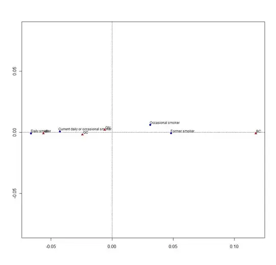
What (I think) should be immediate takeaways are:

1. You are more likely to be a daily smoker if you live in AB, QC, or ON
2. You are more likely to be a former smoker if you live in BC
3. You are least likely to be a daily smoker if you live in BC (this fits with Canadian wide understanding of BC's "active lifestyle" culture)

What could we say about occasional smokers? What would your analysis tell us through this correspondence plot and it's associated summary?

Data Source: Statistics Canada, Canadian Community Health Survey (CCHS 3.1), 2005. The CANSIM table 105-0427 was an update of CANSIM table 105-0227. More current data are in CANSIM tables 105-0501 and 105-0502.

Answer 1

I'm an ecologist, so I apologise in advance is this sounds a bit strange :-)

I like to think of these plots in terms of weighted averages. The region points are at the weighted averages of the smoking status classes and vice versa.

The problem with the above figure is the axis scaling and the fact that you can't display all the relationships (chi-square distance between regions and chi-square distance between smoking status) on the one figure. By the looks of it, the figure is using a what is known as symmetric scaling which has been shown to be a good compromise preserving as much of the information in the sets of scores as possible.

I'm not familiar with the ca package but I am with the vegan package and it's cca function:

require(vegan)
df <- data.frame(df)
ord <- cca(df)
plot(ord, scaling = 3)

The last plot is a bit easier to read than the one you show but AFAICT they are the same (or at least similarly scaled).

So I would say that occasional smokers are lower in number than expected in QC, BC and AB, and most associated with ON, but that in all regions, occasional smokers are low in number - they differ markedly from the expected number.

However, there is a single dominant "gradient" or axis of variation in these data and as the second axis represents so little variation, I would likely not interpret this component at all.