A straightforward way, especially when you expect the points to fall exactly on an ellipse (yet which works even when they don't), is to observe that an ellipse is the set of zeros of a second order polynomial
$$0 = P(x,y) = -1 + \beta_x\,x + \beta_y\,y + \beta_{xy}\,xy + \beta_{x^2}\,x^2 + \beta_{y^2}\,y^2$$
You can therefore estimate the coefficients from five or more points $(x_i,\,y_i)$ using least squares (without a constant term). The response variable is a vector of ones while the explanatory variables are $(x_i,\,y_i, \,x_iy_i,\,x_i^2,\,y_i^2)$.
Here are 60 points drawn with considerable error.
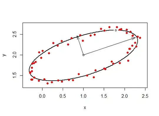
The fit is shown as a black ellipse. The center and axes of the true underlying ellipse are plotted for reference.
When the points are known to fall on an ellipse, you may use any five of the points to estimate its parameters. (When you work out the normal equations you will obtain an explicit formula for the ellipse in terms of those ten coordinates.) It's best to choose the points situated widely around the ellipse rather than clustered in one place.
This is the R code used to do the work. The three lines in the middle after "Estimate the parameters" illustrate the use of least squares to find the coefficients.
center <- c(1,2)
axis.main <- c(3,1)
axis.lengths <- c(4/3, 1/2)
sigma <- 1/20               # Error SD in each coordinate
n <- 60                     # Number of points to generate
set.seed(17)
#
# Compute the axes.
#
axis.main <- axis.main / sqrt(crossprod(axis.main))
axis.aux <- c(-axis.main[2], axis.main[1]) * axis.lengths[2]
axis.main <- axis.main * axis.lengths[1]
axes <- cbind(axis.main, axis.aux)
#
# Generate points along the ellipse.
#
s <- seq(0, 2*pi, length.out=n+1)[-1]
s.c <- cos(s)
s.s <- sin(s)
x <- axis.main[1] * s.c + axis.aux[1] * s.s + center[1] + rnorm(n, sd=sigma)
y <- axis.main[2] * s.c + axis.aux[2] * s.s + center[2] + rnorm(n, sd=sigma)
#
# Estimate the parameters.
#
X <- as.data.frame(cbind(One=1, x, y, xy=x*y, x2=x^2, y2=y^2))
fit <- lm(One ~ . - 1, X)
beta.hat <- coef(fit)
#
# Plot the estimate, the point, and the original axes.
#
evaluate <- function(x, y, beta) {
  if (missing(y)) {
    y <- x[, 2]; x <- x[, 1]
  }
  as.vector(cbind(x, y, x*y, x^2, y^2) %*% beta - 1)
}
e.x <- diff(range(x)) / 40
e.y <- diff(range(y)) / 40
n.x <- 100
n.y <- 60
u <- seq(min(x)-e.x, max(x)+e.x, length.out=n.x)
v <- seq(min(y)-e.y, max(y)+e.y, length.out=n.y)
z <- matrix(evaluate(as.matrix(expand.grid(u, v)), beta=beta.hat), n.x)
contour(u, v, z, levels=0, lwd=2, xlab="x", ylab="y", asp=1)
arrows(center[1], center[2], axis.main[1]+center[1], axis.main[2]+center[2],
       length=0.15, angle=15)
arrows(center[1], center[2], axis.aux[1]+center[1], axis.aux[2]+center[2],
       length=0.15, angle=15)
points(center[1], center[2])
points(x,y, pch=19, col="Red")

