Dose       Survival
1.044316   0.7085001
2.017041   0.2764831
3.042148   0.1498388
4.058954   0.0451514
5.098904   0.0145274
I have two models to fit the data: the exact model and an approximative one:
exactrepair <- function(x, q2, r, p2) { (1+q2*x*(1+p2/q2*r)+x^2*q2^2*(0.5*r+p2/q2*r)+x^3*q2^3*r^2*p2/q2*0.5)*exp(-(1+p2/q2)*q2*x) }
model.repair <- nlsLM(y ~ exactrepair(x, q2, r, p2), data = ds ,start = list(q2 = 1, p2 = 1, r = 1), trace = T, alg = "port", lower= c(0,0,0), upper = c(1,1,1), weights = 1/exp(y))
And the approximative one:
aprox <- function(x, a, b) {  exp(-a*x-b*x^2) }
model.lq <- nlsLM(y ~ aprox(x, a, b), data = ds ,start = list(a = 0.42, b = 0.080), trace = T, alg = "port", lower= c(0,0), upper = c(Inf,Inf), weights = 1/exp(y))
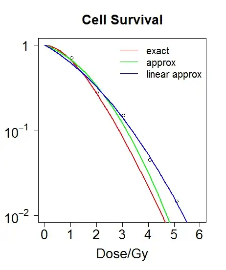
I plotted both the exact and the approximated fits to the data (in red and green respectively).
Now if I take the log of the approx like this:
-In y=a*x+b*x^2
I can fit the data linearly:
aproxlin <- function(x, a, b) {  a*x + b*x^2 }
model12 <- lm(-log(c(1,y))~c(0,x))
If I plot the fitted values from the linear plot I get a much better fit to the data (blue line in the plot).
How can I get better values for the "exact" formula (first version)?
