I have read this article and those linked to it, but I am still having difficulties fitting a function of this form to data I have using the nls function in R. Invariably, I fail to get convergence regardless of what starting values I choose for A through C.
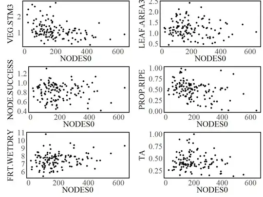
Here is a plot of all six of the relationships I would ultimately like to fit:

While VEG.STM3 and PROP.RIPE probably will conform to a curve of this shape fairly well, the others probably won't, and that's fine. I still have a justifiable reason for trying it.
My questions are as follows:
- What are the parameters
A,B, andCdoing, mathematically, in a function of this form?Aappears to be the Y asymptote,Bseems to be a scalar of some kind, andCseems to control the rate of decay, but, beyond that, I can't seem to figure out what a reasonable range of values for each parameter should be, especially from one set of data to the next. - Is there a way to "linearize" this problem so that
lmcan be used in place ofnls? My understanding is that this function is equivalent toln(Y) ~ ln(A) + ln(B) + CX, but I don't understand how to fit that equation any more than I understand how to fit this current curve. - Is there any way to get
nlsto be less fussy and more robust to lousy starting guesses? - Once I get
nlsto run successfully, how can I compare the fit of the model to one fit by simple linear regression? Would use of AICc be appropriate in that case?
Here is some data to work with:
PROP.RIPE = c(0.37, 0.223, 0.223, 0.224, 0.388, 0.413, 0.406, 0.422, 0.554,
0.453, 0.569, 0.511, 0.13, 0.166, 0.16, 0.216, 0.297, 0.344,
0.339, 0.292, 0.601, 0.535, 0.65, 0.535, 0.269, 0.238, 0.334,
0.272, 0.523, 0.358, 0.449, 0.393, 0.458, 0.426, 0.576, 0.468,
0.581, 0.579, 0.527, 0.568, 0.348, 0.313, 0.317, 0.267, 0.623,
0.527, 0.646, 0.589, 0.488, 0.444, 0.498, 0.449, 0.109, 0.103,
0.171, 0.153, 0.505, 0.343, 0.345, 0.213, 0.029, 0.011, 0.071,
0.013, 0.697, 0.604, 0.624, 0.639, 0.386, 0.508, 0.38, 0.471,
0.618, 0.488, 0.513, 0.485, 0.602, 0.597, 0.625, 0.495, 0.318,
0.457, 0.423, 0.547, 0.88, 0.949, 0.912, 0.771, 0.628, 0.635,
0.486, 0.567, 0.621, 0.549, 0.698, 0.709, 0.541, 0.563, 0.789,
0.692, 0.525, 0.395, 0.449, 0.597, 0.57, 0.487, 0.556, 0.546,
0.495, 0.617, 0.754, 0.71, 0.585, 0.719, 0.508, 0.536, 0.592,
0.472, 0.481, 0.658, 0.937, 0.853, 0.981, 0.887)

NODES0 = c(124L, 362L, 198L, 343L, 152L, 193L, 98L, 167L, 148L, 284L,
113L, 137L, 227L, 323L, 156L, 362L, 166L, 327L, 137L, 312L, 166L,
350L, 97L, 222L, 182L, 456L, 143L, 277L, 172L, 272L, 110L, 184L,
138L, 288L, 102L, 124L, 236L, 280L, 159L, 127L, 104L, 176L, 93L,
167L, 178L, 400L, 126L, 248L, 189L, 336L, 181L, 304L, 245L, 283L,
151L, 327L, 116L, 179L, 144L, 177L, 397L, 642L, 322L, 443L, 125L,
249L, 100L, 144L, 56L, 22L, 23L, 17L, 252L, 387L, 184L, 308L,
115L, 267L, 82L, 157L, 223L, 226L, 79L, 73L, 101L, 139L, 104L,
60L, 200L, 164L, 66L, 49L, 173L, 204L, 64L, 107L, 435L, 215L,
51L, 129L, 392L, 550L, 174L, 178L, 276L, 204L, 98L, 74L, 421L,
303L, 126L, 150L, 168L, 195L, 77L, 75L, 72L, 142L, 59L, 47L,
391L, 479L, 109L, 111L)

NODE.SUCCESS = c(1.05, 0.79, 0.86, 0.69, 0.85, 0.8, 0.77, 0.84, 0.53, 0.88,
0.88, 0.79, 0.85, 0.88, 1, 1.03, 0.95, 0.77, 0.92, 0.73, 0.98,
0.92, 0.97, 0.99, 0.88, 0.82, 0.84, 0.78, 0.63, 0.54, 0.54, 0.47,
1.09, 0.88, 0.95, 0.99, 0.96, 1.13, 0.91, 1.01, 0.81, 0.89, 0.99,
0.85, 0.95, 0.65, 0.87, 0.73, 0.64, 0.82, 0.82, 0.75, 0.93, 1.06,
0.94, 0.89, 0.65, 0.53, 0.6, 0.62, 0.91, 0.89, 0.93, 1.13, 0.81,
0.63, 0.75, 0.67, 0.93, 0.82, 0.7, 0.88, 0.8, 0.96, 0.9, 0.94,
0.58, 0.66, 0.65, 0.63, 0.66, 0.62, 0.66, 0.77, 0.51, 0.6, 0.47,
0.9, 0.69, 0.73, 0.59, 0.63, 0.97, 0.93, 0.95, 0.91, 0.81, 0.92,
0.88, 1.1, 0.56, 0.57, 0.44, 0.51, 0.85, 0.83, 0.96, 0.85, 1,
0.97, 0.94, 0.95, 0.61, 0.71, 0.73, 0.8, 1.06, 0.96, 0.9, 0.91,
0.45, 0.41, 1.3, 0.55)