Mixture of Gaussians on Log of Data

Question

I am practicing Mixture of Gaussians and found the below dataset snoq, which is the precipitation amounts recorded at a US region, with NA and no precipitation days removed.

snoqualmie <- read.csv("http://www.stat.cmu.edu/~cshalizi/402/lectures/16-glm-practicals/snoqualmie.csv",header=FALSE)
snoqualmie.vector <- na.omit(unlist(snoqualmie)) # remove NA's and flatten
snoq <- snoqualmie.vector[snoqualmie.vector > 0] # days where precipitation was greater than 0 

In the exercise code, the instructor fits a mixture of 2 Gaussians to the data with the below code (the plot.normal.components function is given at the end of my question):

if(!require("mixtools")) { install.packages("mixtools");  require("mixtools") }
snoq.k2 <- normalmixEM(snoq, k=2, maxit=100, epsilon=0.01)
plot(hist(snoq,breaks=101),col="grey",border="grey",freq=FALSE,
     xlab="Precipitation (1/100 inch)",main="Precipitation in Snoqualmie Falls")
lines(density(snoq),lty=2)
sapply(1:2,plot.normal.components,mixture=snoq.k2)

The dotted line is the kernel density estimation (on the empirical pdf) and the two black curves are the fitted Gaussians.

Now, I thought the distribution of snoq is similar to that of an exponential distribution, so my first instict here was to log transform the data and then investigate what happens if I try to fit a Mixture of Gaussians on log data rather than the raw data as the instructor did:

log_snoq <-  log(snoq)
log_snoq.k3 = normalmixEM(log_snoq, k=3, maxit=100, epsilon=0.01) # does not converge!
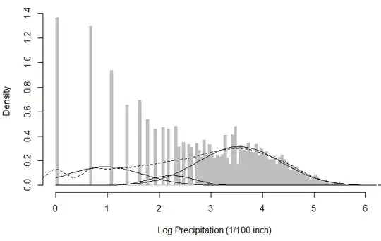
plot(hist(log_snoq,breaks=101),col="grey",border="grey",freq=FALSE,
     xlab="Log Precipitation (1/100 inch)",main="Precipitation in Snoqualmie Falls")
lines(density(log_snoq),lty=2)
sapply(1:3,plot.normal.components,mixture=log_snoq.k3)

I chose k=3 in this case, just because the kernel density estimator showed 3 bumps on the dotted line (in the figure below), which I interpreted as three local maxima that can be modelled by 3 univariate Gaussians. However, during EM I get a warning that says WARNING! NOT CONVERGENT!, and the resulting Gaussian components look as below: (I do realise that the log transform does not produce a beautifully Gaussian-looking distribution, but the raw data itself looks less suitable to be modelled with a (mixture of) Gaussian(s) to me anyway.)

My question is, in this particular example is it wrong to log-transform? Does this in general complicate the application of Mixture of Gaussians? Any recommendations / comments are welcome!

The function plot.normal.components:

plot.normal.components <- function(mixture,component.number,...) {
  curve(mixture$lambda[component.number] *
          dnorm(x,mean=mixture$mu[component.number],
                sd=mixture$sigma[component.number]), add=TRUE, ...)
}

Answer 1

Some comments, advice and answers:

• Unless I'm missing something, I don't fully understand why for some reason you've used different number of mixture components in the second and third blocks of code (3 vs. 2). However, looking at the output of summary() for the mixture object, it seems that the 2nd component is negligible, so I assume that you decided to ignore it, hence the change.
• Warning "NOT CONVERGENT!" can be alleviated in many cases by increasing the number of iterations (for example, I've used the value of 500 instead of the default 100 for my similar analysis). I've tried your code and it converges after 124 iterations, so maxit=200 should be enough.
• I don't think that it's wrong (harmful) to log-transform in this case and it seems that it is even beneficial, as it exposes the structure of the data. However, we definitely need to be careful with log transformations: https://stats.stackexchange.com/a/130275/31372.

Answer 2

Both fitting a mixture of Gaussians to the transformed data and transforming the data prior to fitting appear to be valid approaches, but you may get very different results. Depending on the purpose of your analysis, this may be a problem.

Let's say we are interested in determining the order of a Gaussian mixture. In the example below, we will see that log transforming changes the results (in a dramatic and very boring way):

Let's create an a 2-dimension empirical distribution that is normal on one margin and lognormal on the other:

set.seed(235)
dat<-data.frame(margin1=rnorm(n=10000,mean=21,sd=6),
                margin2=rlnorm(n=10000,meanlog=5))
dat<-dat[dat$margin1>0,] #drop negative values
sample<-dat[sample(rownames(dat),size=3000,replace=TRUE),]

Now let's model it as a mixture of Gaussians:

library(mclust)
sampleBIC<-mclustBIC(sample)

summary(sampleBIC)
             VVI,5        VVI,6        VVE,5
BIC      -58089.92 -58100.22383 -58102.78384
BIC diff      0.00    -10.30452    -12.86453

Using the standard BIC criterion we would select a 5 component mixture model. But look what happens if we log transform the lognormal variable first:

lSample<-data.frame(margin1<-sample$margin1,margin2<-log(sample$margin2))
lSampleBIC<-mclustBIC(lSample)
summary(lSampleBIC)
             EEI,1     EVI,1     VEI,1
BIC      -27781.84 -27781.84 -27781.84
BIC diff      0.00      0.00      0.00

Now BIC would lead us to select a 1 component model.

This makes sense, because by log-transforming the lognormal variable we've given ourselves a roughly bivariate normal joint PDF. At least, "bivariate normal enough" that mclust has no trouble fitting a single elliptical bivariate normal density to it. Before we log-transformed our data, mclust had to fit multiple bivariate gaussians to approximate the observed data, because (even elliptical) bivariate gaussians don't fit very well into the odd asymetrical distribution of our observations.

So it would make sense, here, to think hard about your goal and the interpretability of your results before making the decision to log transform.