Can we use leave one out mean and standard deviation to reveal the outliers?

Question

Suppose I have normally distributed data. For each element of the data I want to check how many SDs it is away from the mean. There might be an outlier in the data (likely only one, but might be also two or three) or not, but this outlier is basically what I am looking for. Does it make sense to temporarily exclude the element I am currently looking at from the calculation of the mean and the SD? My thinking is that if it is close to the mean, it does not have any impact. If it is an outlier, it might bias the calculation of mean and SD and lower the probability that it is detected. I am not a statistician, so any help is appreciated!

Answer 1

It might seem counter-intuitive, but using the approach you describe doesn't make sense (to take your wording, I would rather write "can lead to outcomes very different from those intended") and one should never do it: the risks of it not working are consequential and besides, there exists a simpler, much safer and better established alternative available at no extra cost.

First, it is true that if there is a single outlier, then you will eventually find it using the procedure you suggest. But, in general (when there may be more than a single outlier in the data), the algorithm you suggest completely breaks down, in the sense of potentially leading you to reject a good data point as an outlier or keep outliers as good data points with potentially catastrophic consequences.

Below, I give a simple numerical example where the rule you propose breaks down and then I propose a much safer and more established alternative, but before this I will explain a) what is wrong with the method you propose and b) what the usually preferred alternative to it is.

In essence, you cannot use the distance of an observation from the leave one out mean and standard deviation of your data to reliably detect outliers because the estimates you use (leave one out mean and standard deviation) are still liable to being pulled towards the remaining outliers: this is called the masking effect.

In a nutshell, one simple way to reliably detect outliers is to use the general idea you suggested (distance from estimate of location and scale) but replacing the estimators you used (leave one out mean, sd) by robust ones--i.e., estimates designed to be much less susceptible to being swayed by outliers.

Consider this example, where I add 3 outliers to 47 genuine observations drawn from a Normal 0,1:

n    <- 50
set.seed(123)  # for reproducibility
x    <- round(rnorm(n,0,1), 1)
x[1] <- x[1]+1000
x[2] <- x[2]+10
x[3] <- x[3]+10

The code below computes the outlyingness index based on the leave one out mean and standard deviation (e.g. the approach you suggest).

out_1 <- rep(NA,n)
for(i in 1:n){  out_1[i] <- abs( x[i]-mean(x[-i]) )/sd(x[-i])  }

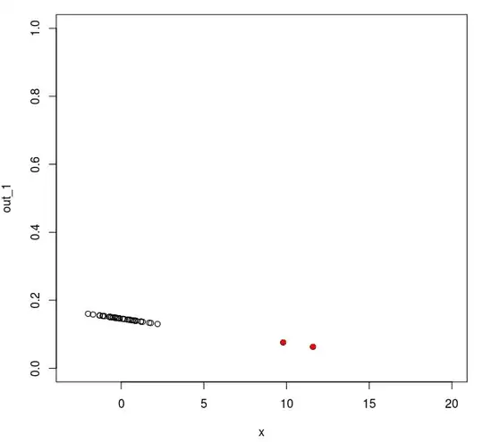
and this code produces the plot you see below.

plot(x, out_1, ylim=c(0,1), xlim=c(-3,20))
points(x[1:3], out_1[1:3], col="red", pch=16)

Image 1 depicts the value of your outlyingness index as a function of the value of the observations (the furthest away of the outliers is outside the range of this plot but the other two are shown as red dots). As you can see, except for the most extreme one, an outlyingness index constructed as you suggest would fail to reveal the outliers: indeed the second and third (milder) outliers now even have a value (on your outlyingness index) smaller than all the genuine observations!...Under the approach you suggest, one would keep these two extreme outliers in the set of genuine observations, leading you to use the 49 remaining observations as if they were coming from the same homogeneous process, giving you a final estimate of the mean and sd based on these 49 data points of 0.45 and 2.32, a very poor description of either part of your sample!

Contrast this outcome with the results you would have obtained using an outlier detection rule based on the median and the mad where the outlyingness of point $x_i$ wrt to a data vector $X$ is

$$O(x_i,X)=\frac{|x_i-\mbox{med}(X)|}{\mbox{mad}(X)}$$

where $\mbox{med}(X)$ is the median of the entries of $X$ (all of them, without exclusion) and $\mbox{mad}(X)$ is their median absolute deviation times 1.4826 (I defer to the linked wiki article for an explanation of where this number comes from since it is orthogonal to the main issue here).

In R, this second outlyingness index can be computed as:

out_2 <- abs( x-median(x) )/mad(x)

and plotted (as before) using:

plot(x, out_2, ylim=c(0,15), xlim=c(-3,20))
points(x[1:3], out_2[1:3], col="red", pch=16)

Image 2 plots the value of this alternative outlyingness index for the same data set. As you can see, now all three outliers are clearly revealed as such. Furthermore, this outlier detection rule has some established statistical properties. This leads, among other things, to usable cut-off rules. For example, if the genuine part of the data can be assumed to be drawn from a symmetric distribution with finite second moment, you can reject all data points for which

$$\frac{|x_i-\mbox{med}(X)|}{\mbox{mad}(X)}>3.5$$

as outliers. In the example above, application of this rule would lead you to correctly flag observation 1,2 and 3. Rejecting these, the mean and sd of the remaining observations is 0.021 and 0.93 receptively, a much better description of the genuine part of the sample!