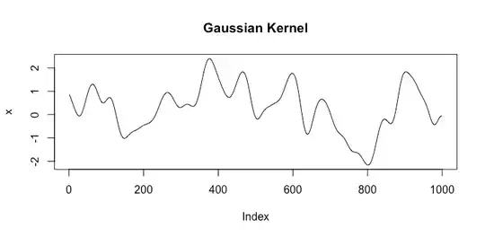
What you mean by defectives is not clear. And what you mean by typical product-to-product variation is not clear. A reasonable solution to your problem requires
clarification on at least one of these points.
Absolute standards to identify defectives. If defectives are typically above or below certain boundaries, then your 'simplistic' method in your item (2) should be just fine. In manufacturing pharmaceutical drugs there is often a baseline of potency (call it 100%) and any lot falling (let's say)
below 80% or above 120% of the standard potency level is automatically discarded. The contents of discarded
batches may actually contain perfectly effective drug, but the irregularity
in production "speaks for itself" and it is deemed too expensive or risky to try
to rescue the non-conforming lots.
If you suspect that 10% of the product may be defective, having extreme values,
a variant of this method might be to sort the data and 'trim' off the top and
bottom 5% of the data, leaving (one hopes) a representative 90% of the sample intact. [This method is the basis of 'trimmed means'.]
Regard outliers as defectives. If you have no reasonable standard and just want to get rid of 'outliers', that is a different problem, which has been "solved" in various ways. One of them is the procedure in your item (1). In your graph getting rid of #13 does make #17
look bad by comparison; and to a lesser extent maybe getting rid of both #13 and #17 makes #4 look 'iffy', and there may be no end to what gets discarded. If high values are 'bad' then it would be unclear where to stop trimming high values
from the sample below from an exponential distribution $(\mu=5).$

Another solution to identifying outliers is to use the outliers often shown in boxplots. It uses the interquartile range (IQR) to measure dispersion. The IQR is the distance between the lower quartile $(Q_1)$ and upper quartile $(Q_3),$ so it spans the 'middle half' of the data. This measure has the advantage of not being sensitive to outliers. Roughly speaking. any observation below $Q_1 - 1.5\text{IQR}$ or above $Q_3 + 1.5\text{IQR}$ is called an outlier.
A difficulty with this method is that such outliers are regular features of some kinds of data: exponential samples almost always have them; even normal $(\mu=100,\, \sigma=15)$ samples characteristically have a few, as shown in the 10 boxplots of samples of size 50
below. [There happen to be more outliers here than usual. About 36% of normal samples of size 50 have outliers, the average number of outliers per sample, among all samples, is about 0.6.]

A third method is described in @User603's link. It uses a different measure of
dispersion that is not sensitive to outliers. Still other methods of identifying items made by a process 'out-of-control' mentioned in @Digio's link may be
applicable.
Minitab statistical software uses a method similar to your item (1) in regression output to
call attention to observations that have 'unusually large residuals'.
The problem with any outlier rule is that individuals tagged as 'outliers' may
not be 'defective'. After some outliers are removed, a second iteration may
tag even more. Even stopping at the first iteration may leave you with a sample
that does not really express the usual range of product-to-product variation.


