3

As I understand it, Pearsons residuals are ordinary residuals expressed in standard deviations.

I ran this Poisson regression:

library(ggplot2)

glm_diamonds <- glm(price ~ carat, family = "poisson", data=diamonds)

I then saved the Pearsons residuals and fitted values from the model:

resid <- resid(glm_diamonds, type = "pearson")
fitted <- fitted(glm_diamonds)
df <- data.frame(resid, fitted)

I then plotted the Pearsons residuals against fitted values:

ggplot(df, aes(fitted, resid)) + geom_point() + ylab("Pearsons residuals") + xlab("Fitted values")

enter image description here

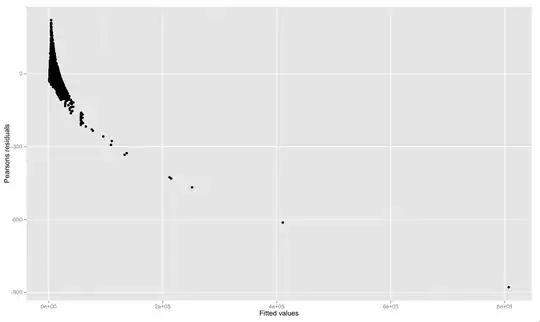
It can be seen in the plot that many of residuals are hundreds of units away from zero. If Pearsons residuals are standard deviations, why are some residuals hundreds of units away from zero? Or in other words, why don't the residuals range from about -3 to 3 if they are standard deviations?

Glen_b
  • 257,508
  • 32
  • 553
  • 939
luciano
  • 12,197
  • 30
  • 87
  • 119
  • As far as I can see, the variable `price` is continuous in this dataset (price in US dollars). This makes the use of Poisson regression questionable. What was your reasoning when choosing Poisson regression? – COOLSerdash May 17 '14 at 12:01
  • I randomly picked a built-in R dataset, without any sort of thinking as to an appropriate model. Question is purely regarding size of Pearsons residuals – luciano May 17 '14 at 12:06
  • The (absolute) residuals are so large because the model fails to fit the observations, obviously. – COOLSerdash May 17 '14 at 12:19
  • I've used Pearsons residuals, not absolute residuals. So if Pearsons residuals are expressed as standard deviations, they should range from about -3 to 3. – luciano May 17 '14 at 12:44
  • 2
    Well, diamonds are usually valued by "the 4 C's" (colour, clarity, cut, carat) - so you have an overdispersion problem without even looking at the data. Also, Poisson has no dispersion parameter, which is like a normal distribution with a fixed variance.. – probabilityislogic May 17 '14 at 13:00
  • 1
    I know that you didn't use absolute residuals. What I meant is that absolute values of Pearson residuals indicate that the model doesn't fit the data very well. Further, the residuals should only fall between -3 to +3 under the assumption that your model is correct. – COOLSerdash May 17 '14 at 13:15
  • So hundreds of prices are hundreds of standard deviations away from their mean value? I'm not in front of R now but the range of the standard deviation of the raw values of `price` are something like -0.9 to 3.5 – luciano May 17 '14 at 13:44
  • 2
    @luciano: Do you know the definition of a Pearson residual? See [here](http://stats.stackexchange.com/questions/99052/) if not. – Scortchi - Reinstate Monica May 17 '14 at 13:49
  • Quite possibly not - see first sentence of question. Would appreciate correction – luciano May 17 '14 at 14:09

2 Answers2

5

The key point is that the standardization method for Pearson residuals is to divide the difference between observed values $y_i$ and the fitted Poisson mean $\hat\mu_i$ by the theoretical standard deviation implied by that fitted mean:

$$r_i=\frac{y_i - \hat\mu_i}{\sqrt{\hat\mu_i}}$$

So if the model is badly mis-specified the assumed relation $\operatorname{Var} \mu_i=\mu_i$ can be wildly inaccurate: you have over-dispersion as @probabilityislogic says; moreover the fitted means are much too large for high-carat stones, indicating the assumed linear relation between the log mean and carat is too simple.

Scortchi - Reinstate Monica
  • 27,560
  • 8
  • 81
  • 248
1

For Poisson regression, you might try using the deviance residual instead of the Pearson residual. Deviance residuals are less biased if there is an unusually high number of zero case counts or mean values that are near-zero. In this case, Pearson is known to underestimate GOF. The likelihood, Pearson, and Deviance for each record are determined as:

${Likelihood}: l_i= \mu_{ij} \log(\hat{\mu}_{ij} / T_{ij}) - \hat{\mu}_{ij}$

${Deviance}: r_D = \mu_{ij} \log(\mu_{ij}/\hat{\mu}_{ij}) + (\hat{\mu}_{ij} - \mu_{ij})$

${Pearson}: r_P = (\mu_{ij} - \hat{\mu}_{ij}) ^ 2 / \hat{\mu}_{ij}=(\mu_{ij} - \hat{\mu}_{ij}) / \sqrt{\hat{\mu}_{ij}}$,

where $d_{ij}$ is the observed number of cases, $\hat{d}_{ij}$ is the expected number of cases, and $T_{ij}$ is the follow-up time. (FYI, in biomedicine, if working with cases or deaths, $d_{ij}=\mu_{ij}$ is the observed number of deaths, and $\hat{d}_{ij}=\hat{\mu}_{ij}$ is the expected number of deaths).

Regarding goodness-of-fit tests, $\sum r_D$, $\sum r_D$ are both $\sim \chi^2_{n-p}$. Thus, if twice the sum of the deviance residuals, $2\sum r_D < \chi^2_{n-p}$, then the model fits. Here $n$ is the number of records, and $p$ is the number of parameters in the model. I have observed many models for which twice the sum of the deviance residuals $2\sum r_D$ was lower than $\sum r_P$.