What does this residuals versus fitted plot mean about my model?

Question

I have a model that attempts to predict a nation's quality of life index by it's moral indifference to contraception and moral rejection of gambling. Initially the model contained several predictors, but I eliminated most using backwards elimination via AIC. Here is a summary of the model (generated using R):

> summary(fit1)

Call:
lm(formula = Quality.of.life.index ~ Morally.unacceptable.ga + 
    Not.a.moral.issue.co, data = qli_and_moral_ind)

Residuals:
    Min      1Q  Median      3Q     Max 
-89.670 -25.443  -4.732  36.129  64.441 

Coefficients:
                        Estimate Std. Error t value Pr(>|t|)    
(Intercept)             143.1410    32.7499   4.371  0.00019 ***
Morally.unacceptable.ga  -1.7690     0.3603  -4.910 4.71e-05 ***
Not.a.moral.issue.co      1.4471     0.7925   1.826  0.07981 .  
---
Signif. codes:  0 ‘***’ 0.001 ‘**’ 0.01 ‘*’ 0.05 ‘.’ 0.1 ‘ ’ 1

Residual standard error: 40.39 on 25 degrees of freedom
Multiple R-squared:  0.6079,    Adjusted R-squared:  0.5765 
F-statistic: 19.38 on 2 and 25 DF,  p-value: 8.266e-06

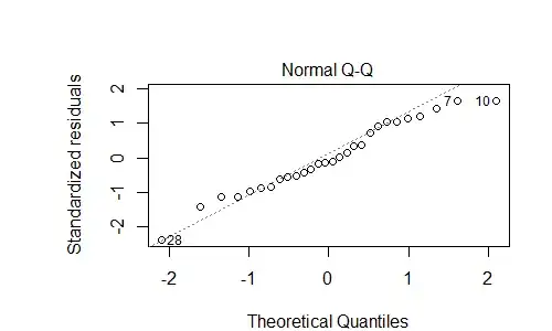
There are two plots of the model that I can't interpret:

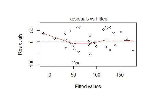
According to the web, the residuals plot above may indicate predictable error, ie that I'm missing some variable in my model. Is that assessment correct? If so, what should I consider adding to the model? It kind of looks like the $y = x^3 - x$ graph - maybe add a cubed term?

Answer 1

The first plot (Normal Q-Q plot) checks if residuals follow a normal distribution, which is an assumption of linear regression. If dots are over the line y=x it means the residuals are normally distributed. Your plot seems OK in this aspect.

The Residuals _versus_ Fitted plot is useful to illustrate if a linear model presents:

1. non-linear relationship between the response variable and predictors.

A horizontal trend line in the plot indicates absence of nonlinear patterns between response and predictors, which is what is expected in a linear model.

2. heteroscedasticity (aka heterogeneity of variance).

A model will exhibit heteroscedasticity when the residuals are not equally spread along the fitted values.

However, as suggested by @BenBolker, a better alternative for visualizing homo/heteroscedasticity is the Scale-Location plot (it uses the Standardized Residuals vs Fitted values) for the reasons written in:

• Trying to understand the fitted vs residual plot?

But why heteroscedasticity is bad?

According to the Wikipedia article:

...the presence of heteroscedasticity can invalidate statistical tests of significance that assume that the modelling errors are uncorrelated and normally distributed and that their variances do not vary with the effects being modelled.

In other words, if one had observed heteroskedasticity, the parameters' standard errors (calculated through t tests) would not make much sense.

Your plot seems to be OK, though.

---

A nice complementary article is Understanding Diagnostic Plots for Linear Regression Analysis from Bommae Kim, University of Virginia.