In cognitive psychology, it has been argued that the learning curve of a skill follows the power function, in which the practice of the skill yields progressively smaller decrements in error. I want to test this hypothesis with the data I have, and to do this I need to fit a power law function to the data.
I heard that the power function can be fit in R by lm(log(y) ~ log(x)). An answer to this post, however, suggests using glm(y ~ log(x), family = gaussian(link = log)), and indeed the resulting fit prefers the (EDIT: See comments. This is not true.).glm approach
# Define a function to compute R-squared in linear space
> rsq <- function(data, fit) {
+ ssres <- sum((data - fit)^2)
+ sstot <- sum((data - mean(data))^2)
+ rsq <- 1 - (ssres / sstot)
+ return(rsq)
}
# generate data and fit a power function with lm() and glm()
> set.seed(10)
> lc <- (1:10)^(-1/2) * exp(rnorm(10, sd=.25)) # Edited
> model.lm <- lm(log(lc) ~ log(1:10))
> model.glm <- glm(lc ~ log(1:10), family = gaussian(link = log))
> fit.lm <- exp(fitted(model.lm))
> fit.glm <- fitted(model.glm)
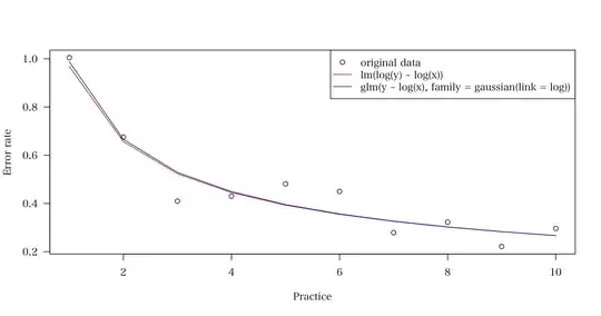
# draw a graph with fitted lines
> plot(1:10, lc, , xlab = "Practice", ylab = "Error rate", las = 1)
> lines(1:10, fit.lm, col = "red")
> lines(1:10, fit.glm, col = "blue")
> legend("topright", c("original data", "lm(log(y) ~ log(x))",
+ "glm(y ~ log(x), family = gaussian(link = log))"),
+ pch = c(1, NA, NA), lty = c(NA, 1, 1), col = c("black", "red", "blue"))
# compute R-squared values for both models
# (EDIT: See comments. These are not good measures to use.)
> rsq(lc, fit.lm)
[1] 0.9194631
> rsq(lc, fit.glm)
[1] 0.9205448
From the $R^2$ values, it seems that the (EDIT: See comments. $R^2$ is not a good measure for this purpose).glm model has a better fit. When the procedure was repeated 100 times, it was always the case that the glm model has a higher $R^2$ value than the lm model
At this point I have two questions.
- What is the difference between the
lmmodel and theglmmodel above? I thought a generalized linear model with the log link function is practically the same as regressing log(y) in general linear models. - I'm trying to compare the fit of the power function against other models (e.g., linear models as in
lm(y ~ x)). To do this, I calculate the fitted values in linear space and compare the $R^2$ values computed in linear space, just like I did to comparelmandglmmodels above. Is this a proper way to compare this type of models?
My final question concerns the estimation of the four-parameter power law function given in this paper (p.186; I modified the notation a little).
$$ E(Y_N) = A + B(N + E)^{-β} $$ where
- $E(Y_N)$ = expected value of $Y$ on practice trial $N$
- $A$ = expected value of $Y$ after learning is completed (i.e., asymptote)
- $E$ = the amount of prior learning before $N = 0$
I have $N$ and $Y$ (1:10 and lc respectively in the code above), and want to estimate $A$, $B$, $E$, and $-β$ from the data. In the example above, I assumed $A$ = $E$ = 0 mostly because I wasn't sure how to estimate four parameters concurrently. While this isn't a huge problem, I would like to estimate $A$ and $E$ from the data as well if possible. So my final question:
- Is there a way to estimate the four parameters in R? If not, is there a way to estimate three parameters, excluding $A$ from the above (i.e., assuming $A$ = 0)?
The paper I linked above says the authors used the simplex algorithm to estimate the parameters. But I am familiar with neither the algorithm nor the simplex function in R.
I'm aware of Clauset et al's work and the poweRlaw package in R. I believe both of them are dedicated to modeling the distribution of one categorical variable, but neither models the curve of the power law.
Any help is appreciated.