Checking residuals for normality in generalised linear models

Question

This paper uses generalised linear models (both binomial and negative binomial error distributions) to analyse data. But then in the statistical analysis section of the methods, there is this statement:

...and second by modelling the presence data using Logistic Regression Models, and the foraging time data using a Generalized Linear Model (GLM). A negative binomial distribution with a log link function was used to model the foraging time data (Welsh et al. 1996) and model adequacy was verified by examination of resi- duals (McCullagh & Nelder 1989). Shapiro–Wilk or Kolmogorov–Smirnov tests were used to test for normality depending on sample size; data were log-transformed before analyses to adhere to normality.

If they assume binomial and negative binomial error distributions, then surely they shouldn't be checking for normality of residuals?

Answer 1

NB the deviance (or Pearson) residuals are not expected to have a normal distribution except for a Gaussian model. For the logistic regression case, as @Stat says, deviance residuals for the $i$th observation $y_i$ are given by

$$r^{\mathrm{D}}_i=-\sqrt{2\left|\log{(1-\hat{\pi}_i)}\right|}$$

if $y_i=0$ &

$$r^{\mathrm{D}}_i=\sqrt{2\left|\log{(\hat{\pi}_i)}\right|}$$

if $y_i=1$, where $\hat{\pi_i}$ is the fitted Bernoulli probability. As each can take only one of two values, it's clear their distribution cannot be normal, even for a correctly specified model:

#generate Bernoulli probabilities from true model
x <-rnorm(100)
p<-exp(x)/(1+exp(x))

#one replication per predictor value
n <- rep(1,100)
#simulate response
y <- rbinom(100,n,p)
#fit model
glm(cbind(y,n-y)~x,family="binomial") -> mod
#make quantile-quantile plot of residuals
qqnorm(residuals(mod, type="deviance"))
abline(a=0,b=1)

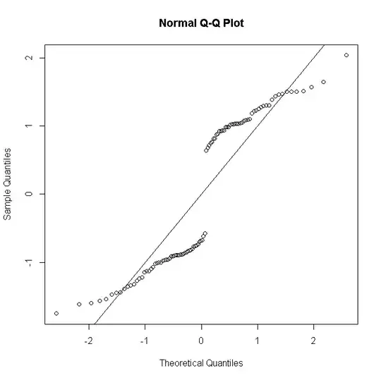
But if there are $n_i$ replicate observations for the $i$th predictor pattern, & the deviance residual is defined so as to gather these up

$$r^{\mathrm{D}}_i=\operatorname{sgn}({y_i-n_i\hat{\pi}_i})\sqrt{2\left[y_i\log{\frac{y_i}{n\hat{\pi}_i}} + (n_i-y_i)\log{\frac{n_i-y_i}{n_i(1-\hat{\pi}_i)}}\right]}$$

(where $y_i$ is now the count of successes from 0 to $n_i$) then as $n_i$ gets larger the distribution of the residuals approximates more to normality:

#many replications per predictor value
n <- rep(30,100)
#simulate response
y<-rbinom(100,n,p)
#fit model
glm(cbind(y,n-y)~x,family="binomial")->mod
#make quantile-quantile plot of residuals
qqnorm(residuals(mod, type="deviance"))
abline(a=0,b=1)

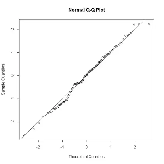
Things are similar for Poisson or negative binomial GLMs: for low predicted counts the distribution of residuals is discrete & skewed, but tends to normality for larger counts under a correctly specified model.

It's not usual, at least not in my neck of the woods, to conduct a formal test of residual normality; if normality testing is essentially useless when your model assumes exact normality, then a fortiori it's useless when it doesn't. Nevertheless, for unsaturated models, graphical residual diagnostics are useful for assessing the presence & the nature of lack of fit, taking normality with a pinch or a fistful of salt depending on the number of replicates per predictor pattern.

Answer 2

What they did is correct! I will give you a reference to double check. See Section 13.4.4 in Introduction to Linear Regression Analysis, 5th Edition by Douglas C. Montgomery, Elizabeth A. Peck, G. Geoffrey Vining. In particular, look at the examples on page 460, where they fit a binomial glm and double check the normality assumption of the "Deviance Residuals". As mentioned on page 458, this is because "the deviance residuals behave much like ordinary residuals do in a standard normal-theory linear regression model". So it make sense if you plot them on normal probability plot scale as well as vs fitted values. Again see page 456 of above reference. In the examples they have provided on page 460 and 461, not only for the binomial case, but also for the Poisson glm and the Gamma with (link=log), they have checked the normality of deviance residuals.
For the binomial case the deviance residual is defined as: $$r^{D}_i=-\sqrt{2|\ln{(1-\hat{\pi_i})}|}$$ if $y_i=0$ and $$r^{D}_i=\sqrt{2|\ln{(\hat{\pi_i})}|}$$ if $y_i=1$. Now some coding in R to show you how you can get it:

> attach(npk)

> #Fitting binomila glm
> fit.1=glm(P~yield,family=binomial(logit))
> 
> #Getting deviance residuals directly
> rd=residuals(fit.1,type = c("deviance"))
> rd
         1          2          3          4          5          6          7 
 1.1038306  1.2892945 -1.2912991 -1.1479881 -1.1097832  1.2282009 -1.1686771 
         8          9         10         11         12         13         14 
 1.1931365  1.2892945  1.1903473 -0.9821829 -1.1756061 -1.0801690  1.0943912 
        15         16         17         18         19         20         21 
-1.3099491  1.0333213  1.1378369 -1.2245380 -1.2485566  1.0943912 -1.1452410 
        22         23         24 
 1.2352561  1.1543163 -1.1617642 
> 
> 
> #Estimated success probabilities
> pi.hat=fitted(fit.1)
> 
> #Obtaining deviance residuals directly
> rd.check=-sqrt(2*abs(log(1-pi.hat)))
> rd.check[P==1]=sqrt(2*abs(log(pi.hat[P==1])))
> rd.check
         1          2          3          4          5          6          7 
 1.1038306  1.2892945 -1.2912991 -1.1479881 -1.1097832  1.2282009 -1.1686771 
         8          9         10         11         12         13         14 
 1.1931365  1.2892945  1.1903473 -0.9821829 -1.1756061 -1.0801690  1.0943912 
        15         16         17         18         19         20         21 
-1.3099491  1.0333213  1.1378369 -1.2245380 -1.2485566  1.0943912 -1.1452410 
        22         23         24 
 1.2352561  1.1543163 -1.1617642 
> 

Check here for the Poisson case as well.