Interpretation of ordinal logistic regression

Question

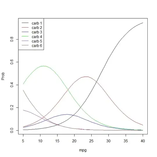
I ran this ordinal logistic regression in R:

mtcars_ordinal <- polr(as.factor(carb) ~ mpg, mtcars)

I got this summary of the model:

summary(mtcars_ordinal)

Re-fitting to get Hessian

Call:
polr(formula = as.factor(carb) ~ mpg, data = mtcars)

Coefficients:
      Value Std. Error t value
mpg -0.2335    0.06855  -3.406

Intercepts:
    Value   Std. Error t value
1|2 -6.4706  1.6443    -3.9352
2|3 -4.4158  1.3634    -3.2388
3|4 -3.8508  1.3087    -2.9425
4|6 -1.2829  1.3254    -0.9679
6|8 -0.5544  1.5018    -0.3692

Residual Deviance: 81.36633 
AIC: 93.36633 

I can get the log odds of the coefficient for mpg like this:

exp(coef(mtcars_ordinal))
 mpg 
0.7917679 

And the the log odds of the thresholds like:

exp(mtcars_ordinal$zeta)

       1|2         2|3         3|4         4|6         6|8 
0.001548286 0.012084834 0.021262900 0.277242397 0.574406353 

Could someone tell me if my interpretation of this model is correct:

As mpg increases by one unit, the odds of moving from category 1 of carb into any of the other 5 categories, decreases by -0.23. If the log odds crosses the threshold of 0.0015, then the predicted value for a car will be category 2 of carb. If the log odds crosses the threshold of 0.0121, then the predicted value for a car will be category 3 of carb, and so on.

Answer 1

You have perfectly confused odds and log odds. Log odds are the coefficients; odds are exponentiated coefficients. Besides, the odds interpretation goes the other way round. (I grew up with econometrics thinking about the limited dependent variables, and the odds interpretation of the ordinal regression is... uhm... amusing to me.) So your first statement should read, "As mpg increases by one unit, the odds of observing category 1 of carb vs. other 5 categories increase by 21%."

As far as the interpretation of the thresholds goes, you really have to plot all of the predicted curves to be able to say what the modal prediction is:

mpg   <- seq(from=5, to=40, by=1)
xbeta <- mpg*(-0.2335)
logistic_cdf <- function(x) {
  return( 1/(1+exp(-x) ) )
}

p1 <- logistic_cdf( -6.4706 - xbeta )
p2 <- logistic_cdf( -4.4158 - xbeta ) - logistic_cdf( -6.4706 - xbeta )
p3 <- logistic_cdf( -3.8508 - xbeta ) - logistic_cdf( -4.4158 - xbeta )
p4 <- logistic_cdf( -1.2829 - xbeta ) - logistic_cdf( -3.8508 - xbeta )
p6 <- logistic_cdf( -0.5544 - xbeta ) - logistic_cdf( -1.2829 - xbeta )
p8 <- 1 - logistic_cdf( -0.5544 - xbeta )

plot(mpg, p1, type='l', ylab='Prob')
  lines(mpg, p2, col='red')
  lines(mpg, p3, col='blue')
  lines(mpg, p4, col='green')
  lines(mpg, p6, col='purple')
  lines(mpg, p8, col='brown')
  legend("topleft", lty=1, col=c("black", "red", "blue", "green", "purple", "brown"), 
         legend=c("carb 1", "carb 2", "carb 3", "carb 4", "carb 5", "carb 6"))

The blue curve for the 3rd category never picked up, and neither did the purple curve for the 6th category. So if anything I would say that for values of mpg above 27 have, the most likely category is 1; between 18 and 27, category 2; between 4 and 18, category 4; and below 4, category 8. (I wonder what it is that you are studying -- commercial trucks? Most passenger cars these days should have mpg > 25). You may want to try to determine the intersection points more accurately.

I also noticed that you have these weird categories that go 1, 2, 3, 4, then 6 (skipping 5), then 8 (skipping 7). If 5 and 7 were missing by design, that's fine. If these are valid categories that carb just does not fall into, this is not good.

Answer 2

In the ordered logit model, the odds form the ratio of the probability being in any category below a specific threshold vs. the probability being in a category above the same threshold (e.g., with three categories: Probability of being in category A or B vs. C, as well as the probability of being in category A vs. B or C).

This leads to the model logit P(Y <= k | x) = zeta_k - eta as specified in the description of polr(). Therefore, odds ratios can be build either for different categories or for different regressors. The latter, the more common one, compares odds for the same categories but different regressors and equals

$$\newcommand{\odds}{{\rm odds}} \frac{\odds(y_a \le k \,|\,x_a)}{\odds(y_b \le k \,|\,x_b)}~=~ \exp(-(\eta_a - \eta_b)).$$

The odds ratio for different categories is defined as

$$\frac{\odds(y_i \le k \,|\,x_i)}{\odds(y_i \le m \,|\,x_i)}~=~ \exp(\zeta_k - \zeta_m),$$

whereby the ratio is independent of the regressors. This property leads to the alternative name proportional odds model.

In this simple, but maybe not very intuitive example, you could formulate: For an one unit increase in the regressor mpg, the odds of observing category 1 vs. observing any higher category (or the odds of observing any category below a certain threshold vs. observing any category above the same threshold) are multiplied by 1.26 or increased by 26% (exp(-(-0.233 - 0)) = 1.263). If you want to formulate an odds ratio of different categories, you could, e.g., say the odds of being in the category 1 vs. any category above compared to the odds of being in category 1 or 2 vs. any category above equals to exp((-6.470) - (-4.415)) = 0.128. Whereby the latter interpretation is not very helpful in this specific setup. An example of an odds ratio for different categories could be the odds of going to college compared to the odds of going to highschool.

Finally, you could be interested how much an explanatory variable must change to reach the next higher response category. For this you compare the interval length $(\zeta_k - \zeta_{k-1})$ with a fitted coefficient. This gives an idea how big the change in your respective regressor must be to move the response from category $k$ to the higher category.