Yes, this is the right approach. Let's see where it can go.
Getting Off to a Fast Start
You can usually sneak up on to a full-blown simulation by working from the inside out. The R command
x <- rcauchy(10, location=0, scale=1)
generates a sample of $10$ and stores it in the variable x. The next step is to compute the statistics of interest. This is why you stored the original output in a variable: so you could use it multiple times without having to regenerate it.
mean(x)
median(x)
sd(x)
etc, etc.
You can go back to the first calculation (of x), repeat it, and recompute its mean and standard deviation (or any other statistic). That's fun and instructive up to a point. For a simulation, though, you will want to repeat these procedures hundreds (or more) times. This is the point at which you want to encapsulate your work into reliable, reusable, flexible components.
Creating the Simulation
R (and many modern computing platforms) work best by generating all the simulated data at once. Let's respect this preference by writing a modular piece of code--a function--to handle both the sample generation and the simulation iterations (which in older languages would require a double loop). Its inputs evidently will include, at a minimum,
n, the sample sizeN, the simulation size (number of samples). Let's default this to $1$ for testing purposes...., any other parameters to be passed to rcauchy.
Here we go:
sim <- function(n=10, N=1, ...) {
  x <- matrix(rcauchy(n*N, ...), nrow=n)             # Each sample is in a separate column
  stats <- apply(x, 2, function(y) c(mean(y), sd(y)))# Compute sample statistics
  rownames(stats) <- c("Mean", "SD")
  return(stats)
}
The reason for giving names to the rows of the output is to help us read it, as in this simulation with three iterations. First the command appears, then its output.
sim(N=3, location=0, scale=1)
          [,1]      [,2]       [,3]
Mean -2.837735  6.471259 0.04831808
SD    4.445549 17.837725 7.00943078
It has been arranged to put all the means in the first row and standard deviations in the second.
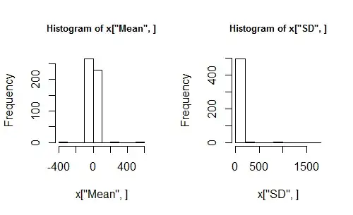
With this in hand, let's run a reproducible simulation by setting the random number seed, generating some statistics for independent random samples, and inspecting them. Let's draw histograms rather than using summary statistics to describe the two rows of output (means and sds).
set.seed(17)
x <- sim(n=10, N=500, location=0, scale=1)
hist(x["Mean", ])
hist(x["SD", ])
(To keep myself honest, I try hard to use the same seed every time for any published results so that people will know I didn't play around with the seed in order to tweak the results to make them look more like I expected! For private exploration I do change the seeds, or leave them unset, so that I see new results each time.)
Using, Re-using, and Extending the Simulation Code
Now you can play.
These histograms look awful. Is it because there weren't enough simulations? Rerun the last four lines of code but change $N$ to $5000$, say. It doesn't help. Change location and scale. Still confused? Maybe we should fall back to a more familiar situation. How about generating Normally distributed samples? To do this, let's just extend our workhorse function sim and let the distribution itself also be a parameter!
sim <- function(n=10, N=1, f=rcauchy, ...) {
  # `f` is any function to generate random variables.  Its first argument must
  # be the number of values to output.
  x <- matrix(f(n*N, ...), nrow=n)                    # Samples are in columns
  stats <- apply(x, 2, function(y) c(mean(y), sd(y))) # Compute sample statistics
  rownames(stats) <- c("Mean", "SD")
  return(stats)
}
The only changes made were to include f=rcauchy in the argument list and to replace the one reference to rcauchy by f. Let's try this with a Normal distribution:
set.seed(17)
x <- sim(n=10, N=5000, f=rnorm, mean=0, sd=1)
par(mfrow=c(1,2)) # Shows two plots side-by-side
hist(x["Mean", ], main="Normal Means")
hist(x["SD", ], main="Normal SDs")
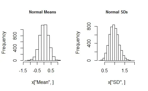
This seems to be working. Now you can vary the distribution, the sample size, the simulation size, and the distribution parameters just by editing the x <- sim(...) line and rerunning it. In a minute or two you should obtain a good sense of how a change of distribution parameters changes the simulation results. With a little more exploration (consider plotting the sequences of means and SDs) you should be able to see why the Cauchy sample distributions seem so messed up.
For studying the Cauchy distribution (and other long-tailed distributions), a good modification to make to sim would be to include sample medians in its output.
Follow-on Analyses
Finally, what about "mean squared errors" (MSE)? These typically are used to compare an estimator to what it is estimating. I recommend storing (in a variable) the value of anything that will be referred to more than once. Thus, for instance, you can study the mean squared error of the mean like this:
location <- 0
x <- sim(n=10, N=5000, f=rcauchy, location=location, scale=1)
mean((x["Mean", ] - location)^2)                              # Mean squared error
Consider stashing the calculation of the MSE within a function if you're going to compute it a lot.
Other assessments of simulation output--plots, descriptive statistics, etc--are just as easily computed because the entire array of relevant simulation output is still available as stored in x.
Going Further: Sources and Principles
For more examples of working simulations in R, search our site for [R] Simulation. Many of these will port nicely to other general-purpose computing platforms like Python, Matlab, and Mathematica. A bit more work might be necessary to port them to specialized statistical platforms like Stata or SAS, but the same principles apply:
Develop the simulation code from the inside out (which is the opposite of good software development practice in general!).
Encapsulate useful blocks of code, such as the simulation code, code to compute the MSE, even code to plot or summarize simulation output.
Respect preferences and idiosyncrasies of the computing environment for best performance (but do not let them dominate your attention: you're doing this to learn about statistics, not about R or Python or whatever).
Extend the functionality of the encapsulated code instead of creating and modifying copies of the original code in order to handle minor variations in what you're doing.
Make the extensions one small step at a time rather than trying to write a do-everything function at the outset.
Use good naming and commenting conventions to document anything that is not immediately clear in the code.
Visualize the output.
Play with your simulations to learn from them. To this end, make them as easy as possible to use and reasonably fast to run.