ancova. I believe the econometric term is difference-in-difference (DID). You may also want to see the Wikipedia pages for ANCOVA and DID, as there may be important differences and assumptions. It's possible to estimate as a general linear model with ordinary least squares, though whether this is optimal will depend on the specific nature of your data. Here's some code for an OLS GLM anyway:
v3=with(data.frame(v2),data.frame(pre=c(pre1,pre2),post=c(post1,post2),
   condition=rep(c(0,1),c(4,4)))) #reorganizing your data into pre-post with a dummy variable
summary(lm(post~scale(pre,scale=F)*condition,v3))  #scaled out nonessential multicollinearity
Results:
Coefficients:                    Estimate Std. Error t value Pr(>|t|)
(Intercept)                      909.6146    40.5553  22.429 2.34e-05 ***
scale(pre, scale = F)              1.0405     0.1096   9.491 0.000688 ***
condition                       -155.9272    57.3534  -2.719 0.053058 .
scale(pre, scale = F):condition   -0.1447     0.1533  -0.943 0.398892

Residual standard error: 81.09 on 4 degrees of freedom
Multiple R-squared:  0.9764,    Adjusted R-squared:  0.9588
F-statistic: 55.24 on 3 and 4 DF,  p-value: 0.001033
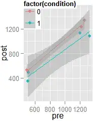
A scatterplot using the ggplot2 package:
 and its code:
ggplot(v3,aes(x=pre,y=post,colour=factor(condition)))+geom_point()+
stat_smooth(method='lm',formula=y~scale(x,scale=F))
Looks like the residuals are bigger for your second group. Test the null hypothesis that they're not, if you like: leveneTest(summary(lm(post~pre,v3))$resid~factor(condition),v3): $F_{(1,6)}=6.2$, $p=.05$.
This heteroscedasticity violates an ANCOVA assumption, but that may not matter greatly (Olejnik & Algina, 1984).
If you want, it's easy to repeat the above after transforming your post scores to ranks (using rank()). The transformation reduces heteroscedasticity $(F_{(1,6)}=2.5,p=.17)$, though the residuals distribute a little less normally. The group difference comes out a little clearer, but the within-subjects differences get obscured slightly:
Coefficients:                 Estimate Std. Error t value Pr(>|t|)
(Intercept)                      5.5488993  0.4110978  13.498 0.000174 ***
scale(pre, scale = F)            0.0054333  0.0011114   4.889 0.008109 **
condition                       -2.0952137  0.5813763  -3.604 0.022680 *
scale(pre, scale = F):condition -0.0002872  0.0015544  -0.185 0.862395
And model fit worsens a little bit:
Residual standard error: 0.822 on 4 degrees of freedom
Multiple R-squared: 0.9357, Adjusted R-squared: 0.8874
F-statistic: 19.39 on 3 and 4 DF,  p-value: 0.007594
And here's that scatterplot: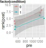 You can see why this emphasizes the group effect relative to the within-subjects effect: ranking wipes out the interaction mostly, and makes the confidence bands evener. Whether this is actually an improvement may depend on your purposes and, again, the specific nature of your data. As for why you shouldn't use an independent-samples $t$ test on change scores, see "Best practice when analysing pre-post treatment-control designs". There's quite a lot of literature on the topic, and even some room for debate, but not within this answer.
Conclusion:
Your two groups appear to have been sampled from different populations. The second group scores lower in general, and lower pre-scores relate to lower post-scores. I see that changes are consistently negative in your second group, and changes in your first group are consistently $\ge0$, but you'd probably want to collect more observations of this difference in the relationship of pre-scores to post-scores across conditions before concluding that the difference in change generalizes to your samples' populations.
Reference
Olejnik, S. F., & Algina, J. (1984). Parametric ANCOVA and the rank transform ANCOVA when the data are conditionally non-normal and heteroscedastic. Journal of Educational and Behavioral Statistics, 9(2), 129–149.