Interaction term in linear regression

Question

I have two variables, and the relationship between them looks like that in this plot:

ggplot(mtcars, aes(wt, mpg)) + geom_point()

The relationship between mpg and wt is best described by entering wt as a quadratic term, like this:

lm(mpg ~ wt + I(wt^2), mtcars)

But what if I want to use wt in an interactions term? Should I include wt, wt^2 or both in the interaction term? So lets say I want to include the interaction of wt with cyl, which one of the below models should I use?

lm(mpg ~ wt*cyl + I(wt^2) , mtcars)
lm(mpg ~ wt + I(wt^2)*cyl , mtcars)
lm(mpg ~ wt*cyl + I(wt^2)*cyl , mtcars)

Answer 1

If there is no theory and you just want to find the best fit, you can have a look at the AIC values of the models.

# run the models
m1 <- lm(mpg ~ wt*cyl + I(wt^2) , mtcars)
m2 <- lm(mpg ~ wt + I(wt^2)*cyl , mtcars)
m3 <- lm(mpg ~ wt*cyl + I(wt^2)*cyl , mtcars)

# compare AIC values
AIC(m1, m2, m3)

The result:

   df      AIC
m1  6 153.7035
m2  6 154.2784
m3  7 153.5813

The third model has the lowest AIC score and is therefore the "best" model.

Of course, this model selection depends on using AIC scores as a criterion. If you use another criterion, e.g., BIC scores, the result can be different:

BIC(m1, m2, m3)

   df      BIC
m1  6 162.4979
m2  6 163.0729
m3  7 163.8415

You have to choose a criterion for the model selection.

Answer 2

I believe interaction effects are potentially meaningful for both linear and quadratic terms, so if you really want to test for both, you should use your third equation, or possibly a variant of it:

with(mtcars, #(so the rest will fit on one line with no scroll bar...)
lm(mpg~scale(wt,scale=F)*scale(cyl,scale=F)+I(scale(wt,scale=F)^2)*scale(cyl,scale=F)))

This version centers the variables before multiplying them to remove nonessential multicollinearity. However, I'm not entirely sure this is useful, as I haven't figured out the "when to center" issue. If you're concerned enough to try to figure that one out for yourself, please let me know if you succeed. Conveniently enough, I've collected some references on a recent answer of mine here. Anyway...

Wrapping the above function in summary() produces the following results:

Coefficients:                                   Estimate Std. Error t value Pr(>|t|)    
(Intercept)                                      19.1432     0.6715  28.508  < 2e-16 ***
scale(wt, scale = F)                             -1.1981     2.0659  -0.580  0.56695    
scale(cyl, scale = F)                            -1.4639     0.4638  -3.156  0.00401 ** 
I(scale(wt, scale = F)^2)                         0.7815     1.2242   0.638  0.52878    
scale(wt, scale = F):scale(cyl, scale = F)        0.1855     1.1180   0.166  0.86948    
scale(cyl, scale = F):I(scale(wt, scale = F)^2)  -0.7646     0.5727  -1.335  0.19338

This much is clear enough: mpg decreases as cyl increases $(b=-1.5)$ when controlling wt. FWIW, only cyl's coefficient differs significantly from zero $(t_{(26)}=-3.2,p=$ $.004)$. Nonetheless, I'll interpret all these coefficients for the sake of demonstration. mpg's relationship with wt is complex in this model, and it depends on cyl. BTW, the only reason cyl's relationship with mpg isn't so complex is that we haven't included a quadratic cyl term or its interaction with the mpg terms – and I don't know what's stopping us, other than my concern for limiting the scope of this answer. Still, the cyl interactions apply to cyl's relationship with mpg too, so that relationship depends on wt too. Specifically, cyl's relationship with mpg becomes less negative as wt increases linearly $(b=.2)$, but more negative as wt$^2$ increases $(b=-.8)$. I.e., more cylinders means burning more gas to travel a mile for cars of similar weight, but there's more of a difference between the lighter cars across cylinder classes (4, 6, & 8) than between heavier cars in this dataset (note I'm not generalizing to cars outside the dataset because most results are insignificant) through both the linear and quadratic interaction terms in the relationship function.

As for wt, there is a decreasing linear relationship $(b=-1.2)$ and an increasing quadratic relationship $(b=.8)$ when controlling for cyl. Otherwise, both depend on cyl: the linear relationship becomes less negative as cyl increases, but the quadratic relationship also becomes less positive $(b=-.8)$. I.e., in this dataset, heavier cars burn more gas per mile traveled, but fuel efficiency drops off most rapidly among the lighter cars, and less rapidly among the heavier cars. As for the cylinder interactions, the linear relationship with fuel inefficiency of the heavier cars is not as bad among those with more cylinders, but the quadratic relationship isn't as good.

For instance, median(mtcars$cyl)$=6$. The cars with 8 cylinders reverse the quadratic relationship with extra weight $(.8\cdot$ wt$^2-.8\cdot2$ wt$^2=-.8\cdot$ wt$^2$, roughly), so fuel efficiency drops off more rapidly with extra weight...though the linear relationship with weight is slightly more merciful in the 8-cylinder class. Conversely, the 4-cylinder class of cars has some super-efficient lightweights, and the heavyweights are relatively even in efficiency among themselves, though much less efficient than the lightweights. Fuel efficiency among the 4-cylinder cars relates more strongly to weight via both the linear negative and quadratic positive terms.

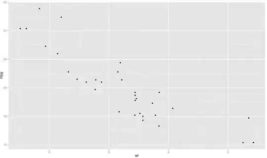
Interactions like these get very confusing. The wise way to sort it out is to produce plots. Here's a three-dimensional plot of this overall model of the mtcars data using WolframAlpha:$y=19.1-1.2x-1.5z+.8x^2+.2xz-.8x^2z$ In this quadratic multinomial function, $x=$ wt $-\mu_\text{wt},\ y=$ mpg, and $z=$ cyl $-\mu_\text{cyl}$. All of this seems very richly informative, but don't be fooled. Once I break this down into three functions of wt for the separate cyl classes and plot them over scatterplots, I think you'll see why only the main effect of cyl was significant: the linear and quadratic trends over wt aren't that strong when considered separately in each cyl class, they really don't vary that dramatically across classes, and several of the too-few data points have nontrivial residuals.

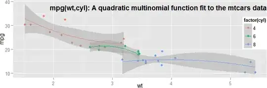
R code for the figure above using the ggplot2 package thanks to UCLA Stat Consulting Group:

ggplot(mtcars,aes(x=wt,y=mpg,colour=factor(cyl)))+geom_point()+
stat_smooth(method='lm',formula=y~scale(x,scale=F)+I(scale(x,scale=F)^2))
title('mpg(wt,cyl): A quadratic multinomial function fit to the mtcars data')

First-timer with ggplot2 here BTW; hope I pulled it off passably! Critiques welcome!

Answer 3

There's a school of thought that suggests you always start with ~wt$^n\cdot$ cyl, then start removing insignificant terms. This specification includes all powers up to $n$ and all interactions. In this case $n=2$, so you start with 5 terms. You never remove lower-order terms before higher-order; e.g. if wt² stays then wt will stay too, if wt $\cdot$ cyl stays then wt and cyl stay too.