There are two possibilities here: scaling the sample range to get an approximate idea of the sample standard deviation, and using the sample range to produce an estimate of the population $\sigma$ (my earlier comment failed to make the distinction clear).
I think your question is asking about the second, but I'll deal with both.
I'll tackle these two in order.
The ratio of sample range ($\max(x) - \min(x)$) to sample standard deviation is sometimes call the studentized range.
So if the middle of the distribution of studentized range was 3, it could make sense to approximate the sample standard deviation from the range by dividing the range by 3.
[Some people are no doubt wondering why we'd bother - after all why not just calculate the standard deviation instead of a noisy approximation of it? Perhaps we're trying to an eyeball estimate from a scatterplot or something, and the range is relatively quick to get by eye. Sometimes we can get the minimum and maximum but not the standard deviation.]
So for the normal distribution, how is the studentized range distributed?
Here are simulated distributions, for 100000 simulations at various sample sizes for normal data:
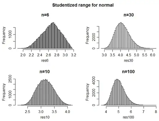
         mean        sd
n=6   2.663658 0.2198905
n=10  3.164088 0.3085827
n=30  4.119035 0.4355710
n=100 5.025396 0.4884935
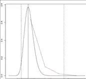
If instead we're trying to estimate the population standard deviation, what matters is the distribution of the range at $\sigma=1$ (since we can work out the distribution for other $\sigma$ is obtained by direct scaling):
          mean        sd
n=6   2.536377 0.8495843
n=10  3.080769 0.8013887
n=30  4.088134 0.6918155
n=100 5.016027 0.6044998
This results in somewhat different distributional shape and different mean and standard deviation (though Slutsky's theorem suggests that as $n$ becomes large they should be more and more similar).
-
The answers to this question discusses the interesting property that at n=6, for many different distributions the range divided by 2.5 provides a reasonable approximation to the standard deviation.
Tippett produced extensive tables of the expected value of the sample range for the standardized normal in 1925 (and briefer tables of the standard deviation and standardized 3rd and 4th moments).
Tippett, L.H.C. (1925),
On the Extreme Individuals and the Range of Samples Taken from a Normal Population,
Biometrika 17 (3-4): 364-387
In either case (approximating $s$ or estimating $\sigma$ for samples from normal distributions), around sample sizes of 8-9, dividing by 3 produces a reasonably good estimate.
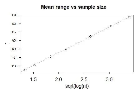
In very large samples, you'd expect a kind of 6-sigma rule to apply, since the "3-sigma" rule is 3 standard deviations either side of the mean. But it's not an asymptotic result since in sufficiently large samples you expect to see the range exceed $6\sigma$. Indeed, by n=1000, we're already close to $6.5\sigma$, and by n=10,000 its near $7.7\sigma$, and for n=100,000 it's somewhere above $8.75\sigma$; the mean of the distribution of the range continues to increase as $n$ increases, but at what appears to be roughly as the square-root of the log of the sample size (that's a pretty slow increase). (Edit indeed, it seems that it's been known for a long time that the growth in mean range is asymptotically proportional to $\sqrt{\log n}$)
Update based on discussion in comments:
It sounds from your comments that the distribution of values are actually reasonably right skew.
I just did a quick simulation to see (at sample size 100) what gamma shape parameter would result in a typical ratio of (max-mean)/(mean-min) of around 1.76 (it turns out to be about $\alpha=7$). So then the question is, for that shape, and at that sample size, how much difference does it make if you use the normal values above?. The somewhat surprising answer is 'hardly any at all'.
You'd want to check at some other sample sizes, but the upshot is - if the actual distribution of values on which your extremes and mean are based is a shifted gamma with shape parameter around 7 (which is moderately skew) - then, at least near n=100, estimates of $\sigma$ you produce from scaling max-min as if they were normal should be about right.
That surprises me that it had even this level of robustness, but it should reassure you a little, at least.
Having repeated the simulation exercise at n=30, and a shape parameter of 7, if the ratio of (max-mean)/(mean-min) doesn't tend to be much larger than 1.76, you should be pretty safe - at least on average - using that normal-based rule to estimate $\sigma$ if the distribution of results isn't much heavier tailed than gamma.