Optimal number of bins in histogram by the Freedman–Diaconis rule: difference between theoretical rate and actual number

Question

Wikipedia reports that under the Freedman and Diaconis rule, the optimal number of bins in an histogram, $k$ should grow as

$$k\sim n^{1/3}$$

where $n$ is the sample size.

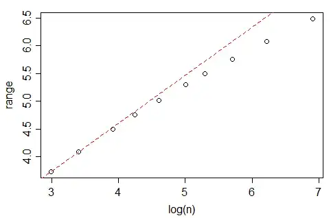
However, If you look at the nclass.FD function in R, which implements this rule, at least with Gaussian data and when $\log(n)\in(8,16)$, the number of bins seems to growth at a faster rate than $n^{1/3}$, closer to $n^{1-\sqrt{1/3}}$ (actually, the best fit suggests $m\approx n^{0.4}$). What is the rationale for this difference?

---

Edit: more info:

The line is the OLS one, with intercept 0.429 and slope 0.4. In each case, the data (x) was generated from a standard gaussian and fed into the nclass.FD. The plot depicts the size (length) of the vector vs the optimal number of class returned by the nclass.FD function.

Quoting from wikipedia:

A good reason why the number of bins should be proportional to $n^{1/3}$ is the following: suppose that the data are obtained as n independent realizations of a bounded probability distribution with smooth density. Then the histogram remains equally »rugged« as n tends to infinity. If $s$ is the »width« of the distribution (e. g., the standard deviation or the inter-quartile range), then the number of units in a bin (the frequency) is of order $n h/s$ and the relative standard error is of order $\sqrt{s/(n h)}$. Comparing to the next bin, the relative change of the frequency is of order $h/s$ provided that the derivative of the density is non-zero. These two are of the same order if $h$ is of order $s/n^{1/3}$, so that $k$ is of order $n^{1/3}$.

The Freedman–Diaconis rule is: $$h=2\frac{\operatorname{IQR}(x)}{n^{1/3}}$$

Answer 1

The reason comes from the fact that the histogram function is expected to include all the data, so it must span the range of the data.

The Freedman-Diaconis rule gives a formula for the width of the bins.

The function gives a formula for the number of bins.

The relationship between number of bins and the width of bins will be impacted by the range of the data.

With Gaussian data, the expected range increases with $n$.

Here's the function:

> nclass.FD
function (x) 
{
    h <- stats::IQR(x)
    if (h == 0) 
        h <- stats::mad(x, constant = 2)
    if (h > 0) 
        ceiling(diff(range(x))/(2 * h * length(x)^(-1/3)))
    else 1L
}
<bytecode: 0x086e6938>
<environment: namespace:grDevices>

diff(range(x)) is the range of the data.

So as we see, it divides the range of the data by the FD formula for bin width (and rounds up) to get the number of bins.

It seems I could have been clearer, so here's a more detailed explanation:
The actual Freedman-Diaconis rule is not a rule for the number of bins, but for the bin-width. By their analysis, the bin width should be proportional to $n^{−1/3}$. Since the total width of the histogram must be closely related to the sample range (it may be a bit wider, because of rounding up to nice numbers), and the expected range changes with $n$, the number of bins is not quite inversely proportional to bin-width, but must increase faster than that. So the number of bins should not grow as $n^{1/3}$ - close to it, but a little faster, because of the way the range comes into it.

Looking at data from Tippett's 1925 tables[1], the expected range in standard normal samples seems to grow quite slowly with $n$, though -- slower even than $\log(n)$:

(indeed, amoeba points out in comments below that it should be proportional - or nearly so - to $\sqrt{\log(n)}$, which grows more slowly than your analysis in the question seem to suggest. This makes me wonder whether there's some other issue coming in, but I haven't investigated whether this range effect fully explains your data.)

A quick look at Tippett's numbers (which go up to n=1000) suggest that the expected range in a Gaussian is very close to linear in $\sqrt{\log(n)}$ over $10\leq n\leq 1000$, but it seems to be not actually proportional for values in this range.

[1]: L. H. C. Tippett (1925). "On the Extreme Individuals and the Range of Samples Taken from a Normal Population". Biometrika 17 (3/4): 364–387