11

I need to draw a complex graphics for visual data analysis. I have 2 variables and a big number of cases (>1000). For example (number is 100 if to make dispersion less "normal"):

x <- rnorm(100,mean=95,sd=50)
y <- rnorm(100,mean=35,sd=20)
d <- data.frame(x=x,y=y)

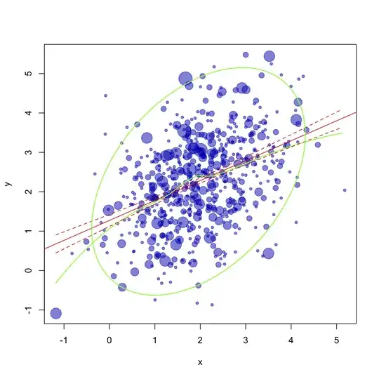
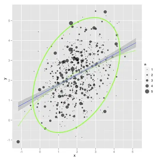
1) I need to plot raw data with point size, corresponding the relative frequency of coincidences, so plot(x,y) is not an option - I need point sizes. What should be done to achieve this?

2) On the same plot I need to plot 95% confidence interval ellipse and line representing change of correlation (do not know how to name it correctly) - something like this:

library(corrgram)
corrgram(d, order=TRUE, lower.panel=panel.ellipse, upper.panel=panel.pts)

correlogramm

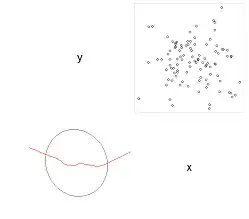
but with both graphs at one plot.

3) Finally, I need to draw a resulting linar regression model on top of this all:

r<-lm(y~x, data=d)
abline(r,col=2,lwd=2)

but with error range... something like on QQ-plot:

QQ-plot

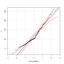
but for fitting errors, if it is possible.

So the question is:

How to achieve all of this at one graph?

Yuriy Petrovskiy
  • 4,081
  • 7
  • 25
  • 30

2 Answers2

30

Does the picture below look like what you want to achieve?

enter image description here

Here's the updated R code, following your comments:

do.it <- function(df, type="confidence", ...) {
  require(ellipse)
  lm0 <- lm(y ~ x, data=df)
  xc <- with(df, xyTable(x, y))
  df.new <- data.frame(x=seq(min(df$x), max(df$x), 0.1))
  pred.ulb <- predict(lm0, df.new, interval=type)
  pred.lo <- predict(loess(y ~ x, data=df), df.new)
  plot(xc$x, xc$y, cex=xc$number*2/3, xlab="x", ylab="y", ...)
  abline(lm0, col="red")
  lines(df.new$x, pred.lo, col="green", lwd=1.5)
  lines(df.new$x, pred.ulb[,"lwr"], lty=2, col="red")
  lines(df.new$x, pred.ulb[,"upr"], lty=2, col="red")    
  lines(ellipse(cor(df$x, df$y), scale=c(sd(df$x),sd(df$y)), 
        centre=c(mean(df$x),mean(df$y))), lwd=1.5, col="green")
  invisible(lm0)
}

set.seed(101)
n <- 1000
x <- rnorm(n, mean=2)
y <- 1.5 + 0.4*x + rnorm(n)
df <- data.frame(x=x, y=y)

# take a bootstrap sample
df <- df[sample(nrow(df), nrow(df), rep=TRUE),]

do.it(df, pch=19, col=rgb(0,0,.7,.5))

And here is the ggplotized version

enter image description here

produced with the following piece of code:

xc <- with(df, xyTable(x, y))
df2 <- cbind.data.frame(x=xc$x, y=xc$y, n=xc$number)
df.ell <- as.data.frame(with(df, ellipse(cor(x, y), 
                                         scale=c(sd(x),sd(y)), 
                                         centre=c(mean(x),mean(y)))))
library(ggplot2)

ggplot(data=df2, aes(x=x, y=y)) + 
  geom_point(aes(size=n), alpha=.6) + 
  stat_smooth(data=df, method="loess", se=FALSE, color="green") + 
  stat_smooth(data=df, method="lm") +
  geom_path(data=df.ell, colour="green", size=1.2)

It could be customized a little bit more by adding model fit indices, like Cook's distance, with a color shading effect.

chl
  • 50,972
  • 18
  • 205
  • 364
  • 1
    @chl +1, nice graph, and short code. – mpiktas Mar 05 '11 at 10:44
  • @mpiktas Thanks. This led me to realize I didn't work with the right sample, in fact :-) – chl Mar 05 '11 at 10:50
  • Almost looks like the one I need, but with real numbers I faced the following problems: 1) `df.new – Yuriy Petrovskiy Mar 05 '11 at 14:36
  • @Yuriy Ok, I will update my code (no need to make any edit in the meantime), but I cannot see how we could get overlap with real-valued random variates with your $(x,y)$ setting; this is the reason why I use boostrap with replacement (this ensures that ~ 2/3 of the original units are present). `car::dataEllipse` does provide the same facilities than in the `ellipse` package, but it is probably less easy to customize. I guess the superimposed curve is just a *loess*, so it is not difficult to add. – chl Mar 05 '11 at 14:56
  • @Yuriy Done. There were two errors in my previous code: (1) as there are replicates in the data.frame, length of `x` and `table(x)` will differ, hence the `cex` param was recycled; (2) I forgot to update the location and scale of the ellipse (not clearly apparent when using standard gaussian variates). I hope there are no other ones. – chl Mar 05 '11 at 16:06
  • Got `Error in ellipse(cor(df$x, df$y), scale = c(sd(df$x), sd(df$y)), centre = c(mean(df$x), : center must be a vector of length 2` and no ellipse :( Everything else is excellent. Thank you very much. – Yuriy Petrovskiy Mar 05 '11 at 16:28
  • @Yuriy It works for me; maybe there's a conflict with another function having the same name (in the car package)? Try to source all the code in a new R session. The picture was generated this way. – chl Mar 05 '11 at 16:35
  • Hi chl, great piece of code. Might I as what does the ellipse actually mean? (p.s: I think I'll repost your answer on my blog, it is a cool piece of code...) – Tal Galili Mar 06 '11 at 14:10
  • 2
    @Tal The interpretation of the ellipse is the same as in the `corrgram` package: it shows 95% pairwise confidence region assuming a bivariate normal distribution centered on the mean and scaled by SD(x) and SD(y). I'm not a big fan of this when used in a scatterplot, though. But see Murdoch & Chow, [A graphical display of large correlation matrices](http://www.jstor.org/pss/2684435), Am Stat (1996) 50:178, or Friendly, [Corrgrams: Exploratory displays for correlation matrices](http://citeseerx.ist.psu.edu/viewdoc/download?doi=10.1.1.19.1268&rep=rep1&type=pdf), Am Stat (2002) 56:316. – chl Mar 06 '11 at 16:01
  • @chl ggplot version is even nicer. It will be better to change colors and line styles: dashed red for ellipse and bolder (dark?)green for loess line... just a suggestion. Nice work. – Yuriy Petr – Yuriy Petrovskiy Mar 06 '11 at 21:27
  • chl, thank you for the explanation (and the links to the papers!), just to be sure - the confidence regions are for the **expectancy** of the bivariate distribution? – Tal Galili Mar 10 '11 at 08:54
  • @Tal Yes, this is always in reference to a theoretical, not empirical, distribution. – chl Mar 10 '11 at 09:59
2

For point 1 just use the cex parameter on plot to set the point size.

For instance

x = rnorm(100)
plot(x, pch=20, cex=abs(x))

To have multiple graphs in one plot use par(mfrow=c(numrows, numcols)) to have an evenly spaced layout or layout to make more complex ones.

nico
  • 4,246
  • 3
  • 28
  • 42
  • 1
    +1 for the tip about `cex`, but I think the OP wants all stuff on the same plotting region, not on separate ones. – chl Mar 05 '11 at 10:28
  • Ahh... now I understand the question. Well, then he can just use `curve` or `points` to overplot the three graphs ;) – nico Mar 05 '11 at 10:54