How could I check if my data e.g. salary is from a continuous exponential distribution in R?
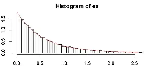
Here is histogram of my sample:
. Any help will be greatly appreciated!
How could I check if my data e.g. salary is from a continuous exponential distribution in R?
Here is histogram of my sample:
. Any help will be greatly appreciated!
I would do it by first estimating the only distribution parameter rate using fitdistr. This won't tell you if the distribution fits or not, so you must then use goodness of fit test. For this, you can use ks.test:
require(vcd)
require(MASS)

# data generation
ex <- rexp(10000, rate = 1.85) # generate some exponential distribution
control <- abs(rnorm(10000)) # generate some other distribution

# estimate the parameters
fit1 <- fitdistr(ex, "exponential")
fit2 <- fitdistr(control, "exponential")

# goodness of fit test
ks.test(ex, "pexp", fit1$estimate) # p-value > 0.05 -> distribution not refused
ks.test(control, "pexp", fit2$estimate) #  significant p-value -> distribution refused

# plot a graph
hist(ex, freq = FALSE, breaks = 100, xlim = c(0, quantile(ex, 0.99)))
curve(dexp(x, rate = fit1$estimate), from = 0, col = "red", add = TRUE)
From my personal experience (though I have never found it officially anywhere, please confirm or correct me), ks.test will only run if you supply the parameter estimate first. You cannot let it estimate the parameters automatically as e.g. goodfit does it. That's why you need this two step procedure with fitdistr.
For more info follow the excellent guide of Ricci: FITTING DISTRIBUTIONS WITH R.
While I'd normally recommend checking exponentiality by use of diagnostic plots (such as Q-Q plots), I'll discuss tests, since people often want them:
As Tomas suggests, the Kolmogorov-Smirnov test is not suitable for testing exponentiality with an unspecified parameter.
However, if you adjust the tables for the parameter estimation, you get Lilliefors' test for the exponential distribution.
Lilliefors, H. (1969), "On the Kolmogorov–Smirnov test for the exponential distribution with mean unknown", Journal of the American Statistical Association, Vol. 64 . pp. 387–389.
The use of this test is discussed in Conover's Practical Nonparametric Statistics.
However, in D'Agostino & Stephens' Goodness of Fit Techniques, they discuss a similar modification of the Anderson-Darling test (somewhat obliquely if I recall right, but I think all the required information on how to approach it for the exponential case is to be found in the book), and that's almost certain to have more power against interesting alternatives.
Similarly, one might estimate something like a Shapiro-Francia test (akin to but simpler than the Shapiro-Wilk), by basing a test on $n(1-r^2)$ where $r$ is the correlation between the order statistics and exponential scores (expected exponential order statistics). This corresponds to testing the correlation in the Q-Q plot.
Finally, one might take the smooth test approach, as in the book by Rayner & Best (Smooth Tests of Goodness of Fit, 1990 - though I believe there's a more recent one, with Thas and "in R" added to the title). The exponential case is also covered in:
J. C. W. Rayner and D. J. Best (1990), "Smooth Tests of Goodness of Fit: An Overview", International Statistical Review, Vol. 58, No. 1 (Apr., 1990), pp. 9-17
Cosma Shalizi also discusses smooth tests in one chapter of his Undergraduate Advanced Data Analysis lecture notes, or see Ch15 of his book Advanced Data Analysis from an Elementary Point of View.
For some of the above, you may need to simulate the distribution of the test statistic; for others tables are available (but in some of those cases, it may be easier to simulate anyway, or even more accurate to simulate yourself, as with the Lilliefors test, due to limited simulation size in the original).
Of all of those, I'd lean toward doing the one that's the exponential equivalent to the Shapiro-Francia (that is, I'd test the correlation in the Q-Q plot [or if I was making tables, perhaps use $n(1-r^2)$, which will reject the same cases] - it should be powerful enough to be competitive with the better tests, but is very easy to do, and has the pleasing correspondence to the visual appearance of the Q-Q plot (one could even choose to add the correlation and the p-value to the plot, if desired).
You can use a qq-plot, which is a graphical method for comparing two probability distributions by plotting their quantiles against each other.
In R, there is no out-of-the-box qq-plot function for the exponential distribution specifically (at least among the base functions). However, you can use this:
qqexp <-  function(y, line=FALSE, ...) {
    y <- y[!is.na(y)]
    n <- length(y)
    x <- qexp(c(1:n)/(n+1))
    m <- mean(y)
    if (any(range(y)<0)) stop("Data contains negative values")
    ylim <- c(0,max(y))
    qqplot(x, y, xlab="Exponential plotting position",ylim=ylim,ylab="Ordered sample", ...)
    if (line) abline(0,m,lty=2)
    invisible()
  }
While interpreting your results: If the two distributions being compared are similar, the points in the q-q plot will approximately lie on the line y = x. If the distributions are linearly related, the points in the q-q plot will approximately lie on a line, but not necessarily on the line y = x.