12

I have a problem with the estimation parameter for Zipf. My situation is the following:

I have a sample set (measured from an experiment that generates calls that should follow a Zipf distribution). I have to demonstrate that this generator really generates calls with zipf distribution. I already read this Q&A How to calculate Zipf's law coefficient from a set of top frequencies? but I reach bad results because i use a truncated distribution. For example if I set the "s" value to "0.9" for the generation process, if I try to estimate "s" value as wrote in the reported Q&A I obtain "s" equal to 0.2 ca. I think this is due to the fact that i use a TRUNCATED distribution (i have to limit the zipf with a truncation point, it is right-truncated).

How can i estimate parameters with a truncated zipf distribution?

Maurizio
  • 265
  • 2
  • 9
  • to be clear, what precisely are you right-truncating? The distribution of values or the Zipf plot itself? Do you know the truncation point? Is the truncation an artifact of the data or an artifact of the *data processing* (e.g., some decision that you or the experimenter made)? Any additional details would be helpful. – cardinal Feb 21 '11 at 17:00
  • @cardinal. (part 1/2) Thanks cardinal. I will give more details: I have a VoIP generator that generates calls following the Zipf (and other distribution) for volume per caller. I have to verify that this generator really follows these distributions. For Zipf Distribution i need to define the truncation point (hence it is known and it refers to the distribution of values) which is the maximum number of generated call by the user and the scale parameter. In particular in my case this value is equal to 500, that indicates that one user can generate maximum 500 calls. – Maurizio Feb 21 '11 at 17:20
  • (part 2/2) The other parameter to set is the scale parameter for Zipf that defines the spread of the distribution (this value in my case is 0.9). I have all the parameters (size of sample, frequency per user, etc.) but i have to verify that my dataset follows the zipf distribution. – Maurizio Feb 21 '11 at 17:21
  • so you're apparently renormalizing the distribution by $\sum_{i=1}^{500} i^{-0.9}$, since for, what I would think of as a "truncated Zipf", a scaling parameter of 0.9 would be impossible. If you can generate lots of these data and you "only" have 500 possible outcomes, why not just use a chi-square goodness-of-fit test? Since your distribution has a long-tail, you may need a pretty large sample size. But, that would be one way. Another quick-and-dirty method would be to check that you get the right empirical distribution for *small* values of the number of calls. – cardinal Feb 21 '11 at 17:40

3 Answers3

15

Update: 7 Apr 2011 This answer is getting quite long and covers multiple aspects of the problem at hand. However, I've resisted, so far, breaking it into separate answers.

I've added at the very bottom a discussion of the performance of Pearson's $\chi^2$ for this example.


Bruce M. Hill authored, perhaps, the "seminal" paper on estimation in a Zipf-like context. He wrote several papers in the mid-1970's on the topic. However, the "Hill estimator" (as it's now called) essentially relies on the maximal order statistics of the sample and so, depending on the type of truncation present, that could get you in some trouble.

The main paper is:

B. M. Hill, A simple general approach to inference about the tail of a distribution, Ann. Stat., 1975.

If your data truly are initially Zipf and are then truncated, then a nice correspondence between the degree distribution and the Zipf plot can be harnessed to your advantage.

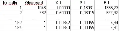
Specifically, the degree distribution is simply the empirical distribution of the number of times that each integer response is seen, $$ d_i = \frac{\#\{j: X_j = i\}}{n} . $$

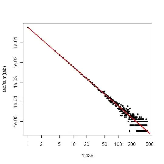
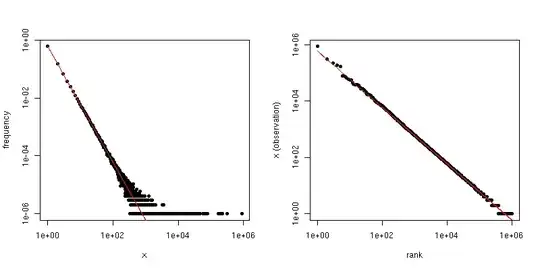
If we plot this against $i$ on a log-log plot, we'll get a linear trend with a slope corresponding to the scaling coefficient.

On the other hand, if we plot the Zipf plot, where we sort the sample from largest to smallest and then plot the values against their ranks, we get a different linear trend with a different slope. However the slopes are related.

If $\alpha$ is the scaling-law coefficient for the Zipf distribution, then the slope in the first plot is $-\alpha$ and the slope in the second plot is $-1/(\alpha-1)$. Below is an example plot for $\alpha = 2$ and $n = 10^6$. The left-hand pane is the degree distribution and the slope of the red line is $-2$. The right-hand side is the Zipf plot, with the superimposed red line having a slope of $-1/(2-1) = -1$.

Degree distribution (left) and Zipf (right) plots for an i.i.d. sample from a Zipf distribution.

So, if your data have been truncated so that you see no values larger than some threshold $\tau$, but the data are otherwise Zipf-distributed and $\tau$ is reasonably large, then you can estimate $\alpha$ from the degree distribution. A very simple approach is to fit a line to the log-log plot and use the corresponding coefficient.

If your data are truncated so that you don't see small values (e.g., the way much filtering is done for large web data sets), then you can use the Zipf plot to estimate the slope on a log-log scale and then "back out" the scaling exponent. Say your estimate of the slope from the Zipf plot is $\hat{\beta}$. Then, one simple estimate of the scaling-law coefficient is $$ \hat{\alpha} = 1 - \frac{1}{\hat{\beta}} . $$

@csgillespie gave one recent paper co-authored by Mark Newman at Michigan regarding this topic. He seems to publish a lot of similar articles on this. Below is another along with a couple other references that might be of interest. Newman sometimes doesn't do the most sensible thing statistically, so be cautious.

MEJ Newman, Power laws, Pareto distributions and Zipf's law, Contemporary Physics 46, 2005, pp. 323-351.

M. Mitzenmacher, A Brief History of Generative Models for Power Law and Lognormal Distributions, Internet Math., vol. 1, no. 2, 2003, pp. 226-251.

K. Knight, A simple modification of the Hill estimator with applications to robustness and bias reduction, 2010.


Addendum:

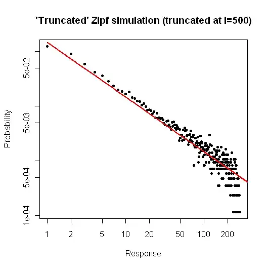
Here is a simple simulation in $R$ to demonstrate what you might expect if you took a sample of size $10^5$ from your distribution (as described in your comment below your original question).

> x <- (1:500)^(-0.9)
> p <- x / sum(x)
> y <- sample(length(p), size=100000, repl=TRUE, prob=p)
> tab <- table(y)
> plot( 1:500, tab/sum(tab), log="xy", pch=20, 
        main="'Truncated' Zipf simulation (truncated at i=500)",
        xlab="Response", ylab="Probability" )
> lines(p, col="red", lwd=2)

The resulting plot is

"Truncated" Zipf plot (truncated at i=500)

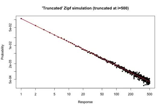
From the plot, we can see that the relative error of the degree distribution for $i \leq 30$ (or so) is very good. You could do a formal chi-square test, but this does not strictly tell you that the data follow the prespecified distribution. It only tells you that you have no evidence to conclude that they don't.

Still, from a practical standpoint, such a plot should be relatively compelling.


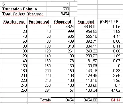
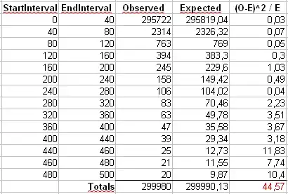
Addendum 2: Let's consider the example that Maurizio uses in his comments below. We'll assume that $\alpha = 2$ and $n = 300\,000$, with a truncated Zipf distribution having maximum value $x_{\mathrm{max}} = 500$.

We'll calculate Pearson's $\chi^2$ statistic in two ways. The standard way is via the statistic $$ X^2 = \sum_{i=1}^{500} \frac{(O_i - E_i)^2}{E_i} $$ where $O_i$ is the observed counts of the value $i$ in the sample and $E_i = n p_i = n i^{-\alpha} / \sum_{j=1}^{500} j^{-\alpha}$.

We'll also calculate a second statistic formed by first binning the counts in bins of size 40, as shown in Maurizio's spreadsheet (the last bin only contains the sum of twenty separate outcome values.

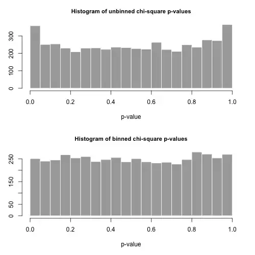
Let's draw 5000 separate samples of size $n$ from this distribution and calculate the $p$-values using these two different statistics.

The histograms of the $p$-values are below and are seen to be quite uniform. The empirical Type I error rates are 0.0716 (standard, unbinned method) and 0.0502 (binned method), respectively and neither are statistically significantly different from the target 0.05 value for the sample size of 5000 that we've chosen.

enter image description here

Here is the $R$ code.

# Chi-square testing of the truncated Zipf.

a <- 2
n <- 300000
xmax <- 500

nreps <- 5000

zipf.chisq.test <- function(n, a=0.9, xmax=500, bin.size = 40)
{
  # Make the probability vector
  x <- (1:xmax)^(-a)
  p <- x / sum(x)

  # Do the sampling
  y <- sample(length(p), size=n, repl=TRUE, prob=p)

  # Use tabulate, NOT table!
  tab <- tabulate(y,xmax)

  # unbinned chi-square stat and p-value
  discrepancy <- (tab-n*p)^2/(n*p)
  chi.stat <- sum(discrepancy)
  p.val    <- pchisq(chi.stat, df=xmax-1, lower.tail = FALSE)

  # binned chi-square stat and p-value
  bins <- seq(bin.size,xmax,by=bin.size)
  if( bins[length(bins)] != xmax )
    bins <- c(bins, xmax)

  tab.bin  <- cumsum(tab)[bins]
  tab.bin <- c(tab.bin[1], diff(tab.bin))

  prob.bin <- cumsum(p)[bins] 
  prob.bin <- c(prob.bin[1], diff(prob.bin))

  disc.bin <- (tab.bin - n*prob.bin)^2/(n * prob.bin)
  chi.stat.bin <- sum(disc.bin)
  p.val.bin <- pchisq(chi.stat.bin, df=length(tab.bin)-1, lower.tail = FALSE)

  # Return the binned and unbineed p-values
  c(p.val, p.val.bin, chi.stat, chi.stat.bin)
}

set.seed( .Random.seed[2] )

all <- replicate(nreps, zipf.chisq.test(n, a, xmax))

par(mfrow=c(2,1))
hist( all[1,], breaks=20, col="darkgrey", border="white",
      main="Histogram of unbinned chi-square p-values", xlab="p-value")
hist( all[2,], breaks=20, col="darkgrey", border="white",
      main="Histogram of binned chi-square p-values", xlab="p-value" )

type.one.error <- rowMeans( all[1:2,] < 0.05 )
cardinal
  • 24,973
  • 8
  • 94
  • 128
  • +1, great answer as usual. You should nominate yourself as a moderator, there is still 1 hour left :) – mpiktas Feb 21 '11 at 18:20
  • @mpiktas, thanks for the compliments and the encouragement. I'm not sure I could justify nominating myself with the already very strong slate of candidates who have, uniformly, participated more extensively and for longer than I have. – cardinal Feb 21 '11 at 18:49
  • @cardinal, here are some links to alternative to Hill's estimator: [original article](http://www.springerlink.com/content/t411403874770047/) by Paulauskas and follow-ups by [Vaiciulis](http://www.springerlink.com/content/4388079545358pn2/) and [Gadeikis and Paulauskas](http://www.springerlink.com/content/f372367226545j25/). This estimator supposedly had better properties than original Hill's. – mpiktas Feb 21 '11 at 20:08
  • @mpiktas, thanks for the links. There are quite a few "new-and-improved" versions of the Hill estimator. The main drawback of the original approach is that it requires a choice of "cutoff" on where to stop averaging. I think mostly that's been done by "eyeballing" it which opens one up to charges of subjectivity. One of Resnick's books on long-tailed distributions discusses this in some detail, if I recall. I think it's his more recent one. – cardinal Feb 21 '11 at 23:30
  • @cardinal, thank you very much, you are very kind and very detailed! Your example in R was very useful for me, but how can I perform a formal chi-square test in this case? (i used chi-square test with other distributions like uniform, exponential, normal, but i have many doubts about the zipf..Sorry but this is my first approach to these topics). Question to modetators: have i to write another Q&A like "how perform chi-square test for truncated zipf distribution?" or continue in this Q&A maybe updating tags and title? – Maurizio Feb 22 '11 at 10:49
  • @Maurizio: In general, you should only edit your question to help clarify details - not ask new questions. This avoids answers referring to past questions. So ask a new question. – csgillespie Feb 22 '11 at 11:45
  • @Maurizio, in principle, chi-square testing in the truncated Zipf case is even easier than for a continuous distribution since you don't need to make any decisions regarding binning, as the data are already discrete. The observed counts are $O_i = n d_i$ and the expected counts are $E_i = n p_i$, where I've calculated the $p_i$ values for you in the $R$ code. From there all you have to do is plug and chug. Hope that helps. – cardinal Feb 22 '11 at 13:44
  • @cardinal, If I could I would offer you a pint of beer! In this afternoon I'll try to do some tests and i'll report my results here. Thank you very much! – Maurizio Feb 22 '11 at 14:08
  • @Maurizio, sorry for the delay in responding. My pleasure. How did things turn out? – cardinal Feb 24 '11 at 00:53
  • @cardinal, I'll post a new answer with the results of my test! – Maurizio Feb 24 '11 at 12:47
5

The paper

Clauset, A et al, Power-law Distributions in Empirical Data. 2009

contains a very good description of how to go about fitting power law models. The associated web-page has code samples. Unfortunately, it doesn't give code for truncated distributions, but it may give you a pointer.


As an aside, the paper discusses the fact that many "power-law datasets" can be modelled equally well (and in some cases better) with the Log normal or exponential distributions!

csgillespie
  • 11,849
  • 9
  • 56
  • 85
  • Unfortunatly this paper does not say anything about the truncated distribution..I found some packages in R that deal with Zipf estimation parameter in a simply way (zipfR, VGAM) but the truncated distribution need a "special treatment". With your last sentence did you mean that it is possible to model a power-law dataset with an e.g. exponential distribution and then apply some estimation parameter process for "truncated" exponential distribution? I'm very newbie in this topic! – Maurizio Feb 21 '11 at 16:27
  • In the paper, the authors re-analyses different data sets where a power-law has been fitted. The authors point out that in a number of cases the power-law model isn't that great and an alternative distribution would be better. – csgillespie Feb 21 '11 at 16:29
2

Following the detailed answer of the user cardinal i performed the chi-square test on my presumable truncated zipf distribution. The results of the chi-square test are reported in the following table:

enter image description here

Where the StartInterval and EndInterval represent for example the range of calls and the Observed is the number of callers generating from 0 to 19 calls, and so on.. The chi-square test is good until the last columns are reach, they increase the final calculation, otherwise until that point the "partial" chi-square value was acceptable!

With other tests the result is the same, the last column (or the last 2 columns) always increases the final value and i don't know why and i don't know if (and how) use another validation test.

PS: for completeness, to calculate the expected values (Expected) i follow cardinal's suggestion in this way:

enter image description here

where X_i's are used to calculate: x <- (1:n)^-S, the P_i's to calculate p <- x / sum(x) and finally the E_i (Expected nr of users for each nr of calls) is obtained by P_i * Total_Caller_Observed

and with Degree of Freedom=13 the Chi-Square goodness rejects always the Hyphotesis that the sample set follow Zipf Distribution because the Test Statistics (64,14 in this case) is larger than that reported in the chi-square tables, "demerit" for the last column. The graphical result is reported here: enter image description here

although the truncation point is set to 500 the maximum value obtaines is 294. I think that the final "dispersion" is the cause of the failure of the chi-square test.

UPDATE!!

I try to perform the chi-square test on a presumable zipf data sample generated with the R code reported in the answer above.

> x <- (1:500)^(-2)
> p <- x / sum(x)
> y <- sample(length(p), size=300000, repl=TRUE, prob=p)
> tab <- table(y)
> length(tab)
[1] 438
> plot( 1:438, tab/sum(tab), log="xy", pch=20, 
        main="'Truncated' Zipf simulation (truncated at i=500)",
        xlab="Response", ylab="Probability" )
> lines(p, col="red", lwd=2)

The associated plot is the following: enter image description here

The chi-square test results are reported in the following figure: enter image description here

and the chi-square test statistic (44,57) is too high for the validation with the chosen Degree of Freedom. Also in this case the final "dispersion" of data is the cause of the high chi-square value. But there is a procedure to validate this zipf distribution (regardless my "wrong" generator, i want to focus on the R data sample) ???

Maurizio
  • 265
  • 2
  • 9
  • @Maurizio, for some reason, I missed this post until now. Is there anyway you can edit it and add a plot similar to the last one in my post, but using your observed data? That might help diagnose the problem. I think I saw another question of yours where you were having trouble producing a uniform distribution, so maybe that is carrying over into these analyses as well. (?) Regards. – cardinal Mar 02 '11 at 00:45
  • @cardinal, I updated the results! What do you think? The question about the uniform distribution is another thing that i have to specify in a better way and i ll do it today or tomorrow ;) – Maurizio Mar 07 '11 at 14:41
  • @Maurizio, were these generated randomly? Was your scale parameter $S = 0.9$ as before? I used a sample size of 8454 and a truncation point of 500 and generated 10000 such samples. Of these 10000, the maximum observed value in the sample was 500 for 9658 of the trials, 499 for 324 trials, 498 for 16 trials and 497 for 2 trials. Based on this, I think something is still wrong with your generation procedure. Unless you used a different scale parameter. – cardinal Mar 13 '11 at 03:54
  • @Maurizio, to explain the results I posted, consider that $p = \mathbb{P}(X_i = 500) \approx 4.05 \times 10^{-4}$. So, in a sample size of $n = 8454$, the expected number of outcomes with the value 500 is $8454 \cdot 4.05 \cdot 10^{-4} \approx 3.43$. The probability of seeing *at least* one such outcome is $1 - (1 - 0.000405)^{8454} \approx 0.9675$. Note how closely that matches up to the simulation above. – cardinal Mar 13 '11 at 15:28
  • @cardinal, i also think that there is something "wrong" in the generation procedure (my goal is to validate that this generator really follows the Zipf distribution). I have to speak with the designers of the project in these days. – Maurizio Mar 14 '11 at 13:15
  • @cardinal, But i have a question about your example. If I perform the chi-square test (as you have suggested to me in your posts) on a sample data generated with your R code i obtain an high value result that lead me to reject the hypothesis that the data sample is following a zipf distribution. In particular i used SCALE = 2, SIZE = 300000, TRUNCATION = 500. I'll update this answer with the chi-square results! – Maurizio Mar 14 '11 at 13:16
  • @Maurizio, see my updated answer. I've done a simulation study on two different chi-square statistics, including the one that you show above using the same values for the scale parameter, sample size, and truncation point. Using my code to generate the truncated Zipf, I get that the chi-square tests give very sensible results, with a Type I error very close to 0.05. So, I think you may be doing something wrong. Also, you might consider accepting an answer if you think one of them provides enough useful information. – cardinal Apr 08 '11 at 01:53