What distribution to fit if the log of log is still convex?

Question

I am trying to fit a model with variable x, and y. plot(x, y) shows that it is convex (downward) and decaying which makes me think I need to make a log transformation of y, but plot(x, log(y)) is still convex, even more plot(x, log(log(y))), plot(x, log(log(log(y)))) are also convex, what kind of model should I fit to this?

How does my data comes from?

Say I have a feature which takes only integer value from 1 to some big int here, I would like to see what distribution this feature follows, so I make a simple count of the feature, CatX would be the feature's value, 1,2,3,etc. CntY would be how many times the value occurs in my data:

Fit the model?

I am trying to understand the underlying distribution of my feature, but I have very rough statistic knowledge, so what distribution should this belong to?

This is a direct plot of CntY ~ CatX:

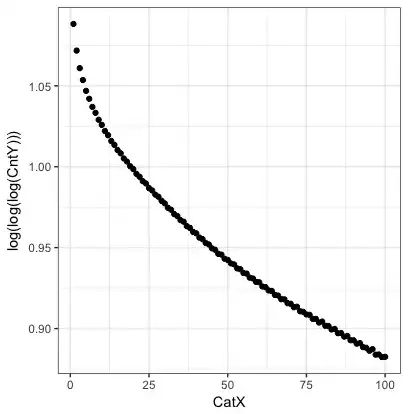
This is a plot of log(log(log(CntY))) ~ CatX:

What is your modeling goal? And can you post a plot of the data? — shadowtalker, Jan 12 '17 at 18:49
Some description of your data would be helpful. There's nothing about your plot, for instance, that would rule out the interpretation that "X" is not a variable at all and that you have simply plotted the values of $Y$ in descending order (although I wonder about the tiny blips near $X=72$ and $X=96$). Please, then, explain what you mean by "fit a model." — whuber, Jan 12 '17 at 19:26
@whuber Thanks for the response. I added some explanation here, hopefully it makes some sense. The real case is that my data is large, so I made some transformation before plotting. `X` is the actual values the feature takes and it's numeric nature, so the plot is not by descending order of Y but ascending order of X. — Psidom, Jan 12 '17 at 19:36
$X$ and $Y$ are not separate variables. You're asking about modeling the frequency distribution of $X$. — shadowtalker, Jan 12 '17 at 19:40
@ssdecontrol That's correct. I made them as two to compress the data size so that I can visualize and analyze them on my laptop. — Psidom, Jan 12 '17 at 19:42
Plot $y$ vs $x$ on log-log axes, then read about the [Zipf distribution](http://stats.stackexchange.com/questions/7450). — whuber, Jan 12 '17 at 20:27

score 7 · Accepted Answer · edited Apr 13 '17 at 12:44

It is plausible these data follow a Zipf distribution.

Here, for comparison, are random data generated according to a Zipf (power-law) distribution with power near $-1.4$ and plotted as in the question and the linked discussion. I have tuned the power and the total frequencies to match the figures in the question--the match looks pretty good in the raw plot of ordered frequencies (at left) and the (untitled) log-log-log plot (second from left).

A good way to analyze data that look like this is to display frequency against rank on log-log axes, as shown in the "Zipf Plot" above. Even if it turns out these data are not Zipf distributed, a comparison to a Zipf distribution (as exhibited in the "Observed vs. Fit" plot at the right) is likely to be informative.

More information about these figures can be gleaned from the R code used to generate them.

x <- 1:100
Y <- exp(19.5 - 1.392 * log(x))
Y <- round(Y + rnorm(length(Y), sqrt(Y)))

par(mfrow=c(1,4))
plot(x,Y,pch=19, main="Ordered Frequencies")
abline(h=seq(5e7, 3e8, by=5e7), col="Gray")
abline(v=seq(0, 100, by=25), col="Gray")

plot(x, log(log(log(Y))), pch=19)
abline(h=seq(0.925, 1.10, by=0.025), col="Gray")
abline(v=seq(0, 100, by=25), col="Gray")

plot(x, Y, log="xy", main="Zipf Plot")
beta.hat <- coef(lm(log(Y) ~ I(log(x))))
curve(exp(beta.hat[1]+beta.hat[2]*log(x)), add=TRUE, col="Red")

H <- sum(Y)/sum(x^(beta.hat[2]))
plot(H*x^(beta.hat[2]), Y, log="xy",
     ylab="Observed Frequency", xlab="Fitted Frequency",
     main="Observed vs. Fit")
abline(c(0,1), col="Red")

What distribution to fit if the log of log is still convex?

1 Answers1