I will walk through how I generated the exact statistics for the $\chi^2$ distribution and (hopefully) update later with a paper that gives tables for the exact distributions and where the exact distribution converges to the theoretical $\chi^2$ with $6$ degrees of freedom. Ditto for the K-S and Kuiper distributions that ttnphns mentions.
So the steps to generate the exact distributions are:
- Generate all potential combinations of outcomes allocating crimes into the $7$ weekday bins. The total number of combinations ends up being $\binom{M + N - 1}{M - 1}$ where $M = 7$ weekday bins and $N$ equals the number of crimes observed.
- For each of the combinations, calculate the probability of observing that outcome under the null hypothesis. Here the null is that each crime has a multinomial distribution in which the weekdays are the outcomes and are equi-probable (e.g. each day has a probability of $1/7$ of being selected).
- Generate the test statistic for that set of observations.
From this information you can generate critical values for the test distributions under the null. So If you observe $3$ crimes, with two occurring on Monday and one on Tuesday, the probability of that event under the null is:
$$Pr(\text{Mon.} = 2, \text{Tues.} = 1) = \frac{3!}{2!1!} \cdot ({P_m}^2)({P_t}^1) = 0.00874635568513119$$
Where $P_m$ and $P_t$ symbolize the probability of an event on Monday and Tuesday respectively, and $P_m = P_t = 1/7$. (If you wanted to generalize to a window in which say spans 10 days, you may want to consider unequal probalities of $2/10$ for the overlapping days and $1/10$ for the others.)
For an example of generating the exact distribution of the test statistic, with three crimes there are only three different possible $\chi^2$ values out of the 84 different combinations (since order doesn't matter for the statistic). The below table symbolizes these potential outcomes. (Just imagine sorting the days of the week so the day of the week with the most events is in the left most column.)
A  B   C
.
.  .
.  ..  ...
Subsequently, combinations of A appear 7 times, B 42 times, and C 35 times. The below table shows the probabilties of obtaining said $\chi^2$ statistics and how to generate the CDF of the null hypothesis. From here you can see that it is actually possible to reject the null at a .05 critical level if all three events are observed on the same day.
    #  ChiSq    Prob(Sum) CDF
C  35    4         .61    .61
B  42    8.67      .37    .98
A   7   18         .02   1.0
Also from the set of all potential combinations you can generate the distributions under various alternative hypotheses, and this allows you to evaluate the power of the test under those circumstances. So for example for $5$ crimes, the exact $\chi^2$ distribution has a $.05$ critical value at $10.4$. So for an alternative hypothesis of data having positive probability in only two days, you have 100% power (i.e. the only observable $\chi^2$ values if 5 crimes occur in 2 or fewer days of the week is over $10.4$).
The image below shows the CDFs for the exact $\chi^2$ distribution with $5$ crimes in $7$ weekday bins (in light grey lines), CDFs for different alternative hypotheses in dark grey lines, and the critical value $\chi^2$ highlighted with a red guideline. The alternative hypotheses are for differing numbers of days that are equi-probable for the crimes to occur on for $1$ to $4$ days during the week.
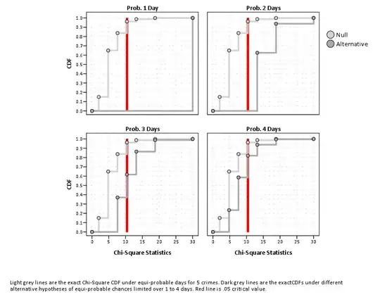
You can see from this chart even for an alternative of equi-probable chances over three days for just 5 crimes the power is just under 40%, 1 minus the CDF of the alt. hypothesis where it intersects the critical value. (Earlier I wrote that a tie goes to rejecting the null, but that would be incorrect as the Type 1 error would be inflated to .39 instead of .02 in my 3 crimes example.)
I have a paper going through this same analysis and generating critical values for Kuiper's $V$ and the $\chi^2$ test now posted on SSRN, Testing for Randomness in Day of Week Crime Sprees with Small Samples.