Best way to visually present relationships from a multiple linear model

Question

I have a linear model with about 6 predictors and I'm going to be presenting the estimates, F values, p values, etc. However, I was wondering what would be the best visual plot to represent the individual effect of a single predictor on the response variable? Scatterplot? Conditional Plot? Effects plot? etc? How would I interpret that plot?

I'll be doing this in R so feel free to provide examples if you can.

EDIT: I'm primarily concerned with presenting the relationship between any given predictor and the response variable.

Do you have interaction terms? Plotting would be much harder if you have them. — Hotaka, Sep 29 '13 at 22:22
You already have six regression coefficients, one for each predictor, which are likely going to be presented in tabular form, what's the reason of repeating the same point again with graph? — Penguin_Knight, Sep 29 '13 at 23:24
For non-technical audiences, I'd rather show them a plot than talk about estimation or how the coefficients are calculated. — AMathew, Sep 30 '13 at 00:00
@tony, I see. Perhaps these two websites can give you some inspiration: using [R visreg package](http://myweb.uiowa.edu/pbreheny/publications/visreg.pdf) and [error bar plot](http://www.r-statistics.com/2010/07/visualization-of-regression-coefficients-in-r/) to visualize regression models. — Penguin_Knight, Sep 30 '13 at 00:46
I have had some success in presenting the change in model AIC upon the dropping of each predictor variable in your final model (i.e. `drop1()`). This gives an indication as to the significance of each variable. A bar plot of these delta AIC values can help "pop out" the importance of terms visually - i.e. those terms whose removal causes the highest increase in AIC are the most important. — Marc in the box, Sep 30 '13 at 12:54

score 12 · Accepted Answer · edited Feb 16 '17 at 19:30

In my opinion, the model that you've described doesn't really lend itself to plotting, as plots function best when they display complex information that is hard to understand otherwise (e.g., complex interactions). However, if you'd like to display a plot of the relationships in your model, you've got two main options:

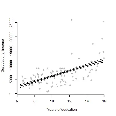
Display a series of plots of the bivariate relationships between each of your predictors of interest and your outcome, with a scatterplot of the raw datapoints. Plot error envelopes around your lines.
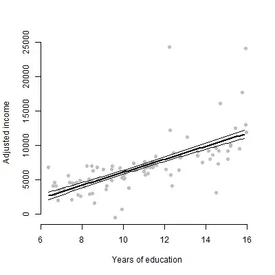
Display the plot from option 1, but instead of showing the raw datapoints, show the datapoints with your other predictors marginalized out (i.e., after subtracting out the contributions of the other predictors)

The benefit of option 1 is that it allows the viewer to assess the scatter in the raw data. The benefit of option 2 is that it shows the observation-level error that actually resulted in the standard error of the focal coefficient that you're displaying.

I have included R code and a graph of each option below, using data from Prestige dataset in the car package in R.

## Raw data ##

mod <- lm(income ~ education + women, data = Prestige)
summary(mod)

# Create a scatterplot of education against income
plot(Prestige$education, Prestige$income, xlab = "Years of education", 
     ylab = "Occupational income", bty = "n", pch = 16, col = "grey")
# Create a dataframe representing the values on the predictors for which we 
# want predictions
pX <- expand.grid(education = seq(min(Prestige$education), max(Prestige$education), by = .1), 
                  women = mean(Prestige$women))
# Get predicted values
pY <- predict(mod, pX, se.fit = T)

lines(pX$education, pY$fit, lwd = 2) # Prediction line
lines(pX$education, pY$fit - pY$se.fit) # -1 SE
lines(pX$education, pY$fit + pY$se.fit) # +1 SE

Graph using raw datapoints

## Adjusted (marginalized) data ##

mod <- lm(income ~ education + women, data = Prestige)
summary(mod)

# Calculate the values of income, marginalizing out the effect of percentage women
margin_income <- coef(mod)["(Intercept)"] + coef(mod)["education"] * Prestige$education + 
    coef(mod)["women"] * mean(Prestige$women) + residuals(mod)

# Create a scatterplot of education against income
plot(Prestige$education, margin_income, xlab = "Years of education", 
     ylab = "Adjusted income", bty = "n", pch = 16, col = "grey")
# Create a dataframe representing the values on the predictors for which we 
# want predictions
pX <- expand.grid(education = seq(min(Prestige$education), max(Prestige$education), by = .1), 
              women = mean(Prestige$women))
# Get predicted values
pY <- predict(mod, pX, se.fit = T)

lines(pX$education, pY$fit, lwd = 2) # Prediction line
lines(pX$education, pY$fit - pY$se.fit) # -1 SE
lines(pX$education, pY$fit + pY$se.fit) # +1 SE

Adjusted data

Best way to visually present relationships from a multiple linear model

1 Answers1

Linked