How does the beta prior affect the posterior under a binomial likelihood

Question

I have two questions,

Question 1: How can I show that the posterior distribution is a beta distribution if the likelihood is binomial and the prior is a beta

Question 2: How does choices the prior parameters affect the posterior? Shouldn't they all be the same?

Is it possible to answers these questions in R?

Answer 1

To answer your first question we just need to use Bayes' Theorem to update our binomial likelihood with the beta prior. To better understand how to do this, first observe the following result $$p(\theta|\mathbf{x})=\frac{p(\mathbf{x}|\theta)p(\theta)}{\int_{\Theta}p(\mathbf{x}|\theta)p(\theta)d\theta}\propto p(\mathbf{x}|\theta)p(\theta)$$ where we can make use of the proportionality result since the beta distribution is the conjugate prior for the binomial likelihood.

Now, let $x_i\sim\text{Binomial}(N_i,\theta)$ and $\theta\sim\text{Beta}(\alpha,\beta)$. We can now use Bayes' Theorem to calculate the posterior as follows:

\begin{align} p(\theta|\mathbf{x})&\propto p(\mathbf{x}|\theta)p(\theta)\\ &\\ &\propto \binom{N}{x_i}\theta^{s}(1-\theta)^{N-s}\frac{\Gamma(\alpha+\beta)}{\Gamma(\alpha)\Gamma(\beta)}\theta^{\alpha-1}(1-\theta)^{\beta-1}\\ &\\ &\propto \theta^{s}(1-\theta)^{N-s}\theta^{\alpha-1}(1-\theta)^{\beta-1}\\ &\\ &\propto\theta^{\alpha+s-1}(1-\theta)^{\beta+N-s-1} \end{align} where $s=\sum_{i=1}^nx_i$ and $N=\sum_{i=1}^nN_i$

Now, we recognize the proportional right hand side of the equation as the kernel of another beta distribution with updated parameters $$\alpha^*=\alpha+\sum_{i=1}^nx_i$$ and $$\beta^*=\beta+\sum_{i=1}^nN_i-\sum_{i=1}^nx_i$$

Now for the second part of your problem, consider the following graphs of the posteriors given differing prior distributions.

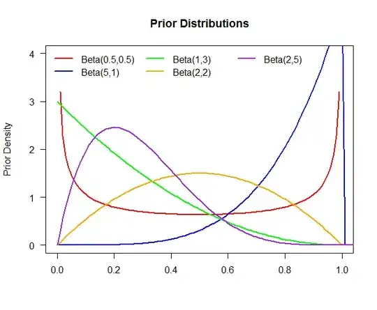
The above plot is of five different prior distributions: \begin{align*} \text{Prior }1&:\,\,\theta\sim\text{Beta}(.5,.5)\\ \text{Prior }1&:\,\,\theta\sim\text{Beta}(5,1)\\ \text{Prior }1&:\,\,\theta\sim\text{Beta}(1,3)\\ \text{Prior }1&:\,\,\theta\sim\text{Beta}(2,2)\\ \text{Prior }1&:\,\,\theta\sim\text{Beta}(2,5) \end{align*}

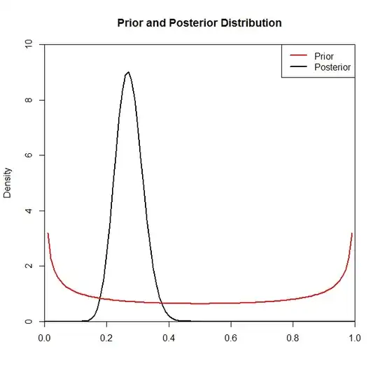
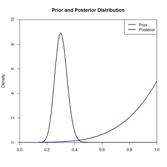
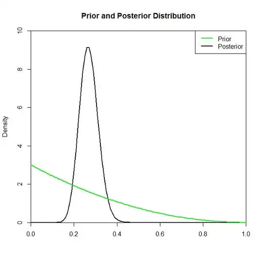
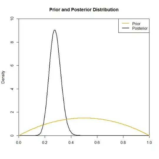
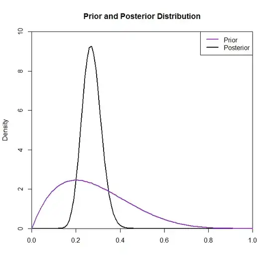
Now although the posterior distribution does not seem to be changed much by the choice of prior in this situation this is not always the case. For example, had we sampled from a Binomial distribution (in the code) where $N=2$ we would see that the posterior distribution is drastically changed by the choice of the prior distribution.

Here is the R code used to generate everything:

colors = c("red","blue","green","orange","purple")

n = 10
N = 10
theta = .2

x = rbinom(n,N,theta)
grid = seq(0,2,.01)


alpha = c(.5,5,1,2,2)
beta = c(.5,1,3,2,5)

plot(grid,grid,type="n",xlim=c(0,1),ylim=c(0,4),xlab="",ylab="Prior Density",
     main="Prior Distributions", las=1)
for(i in 1:length(alpha)){
    prior = dbeta(grid,alpha[i],beta[i])
    lines(grid,prior,col=colors[i],lwd=2)
}

legend("topleft", legend=c("Beta(0.5,0.5)", "Beta(5,1)", "Beta(1,3)", "Beta(2,2)", "Beta(2,5)"),
       lwd=rep(2,5), col=colors, bty="n", ncol=3)

for(i in 1:length(alpha)){
    dev.new()
    plot(grid,grid,,type="n",xlim=c(0,1),ylim=c(0,10),xlab="",ylab="Density",xaxs="i",yaxs="i",
    main="Prior and Posterior Distribution")

    alpha.star = alpha[i] + sum(x)
    beta.star = beta[i] + n*N - sum(x)
    prior = dbeta(grid,alpha[i],beta[i])
    post = dbeta(grid,alpha.star,beta.star)

    lines(grid,post,lwd=2)
    lines(grid,prior,col=colors[i],lwd=2)
    legend("topright",c("Prior","Posterior"),col=c(colors[i],"black"),lwd=2)

}